Recognizing Cats and Dogs With TensorFlow

Using TensorFlow to recognize Cats and Dogs

Use a Convolution Deep Neural Network to enter Kaggle’s Dogs vs Cats competition

I like to use practical examples and projects to help me memorize the theory during my study of Deep Neural Networks. An excellent resource for finding these practical projects is Kaggle. Kaggle is an online community of data scientists and machine learning practitioners.

Kaggle allows you to search and publish data sets, explore, and build models. You can perform these functions in a web-based environment. Kaggle also offers machine learning competitions with actual problems and provides prizes to the winners.

I am currently studying Deep Learning with TensorFlow. One of the subjects I want to learn is image recognition. This article describes my attempt to solve a former Kaggle competition from 2013, called “Dogs vs. Cats.” For implementing the solution I used Python 3.8 and TensorFlow 2.3.0.

The original “Dogs vs. Cats” competition’s goal was to write an algorithm to classify whether images contain either a dog or a cat. Note that in 2013 there was no TensorFlow or another framework such as PyTorch to help.

Although the competition is finished, it is still possible to upload and let Kaggle score your predictions.

Preparing the training data

Before we can create and train a model, we must prepare the training data. The training data for this competition involves 25,000 images of dogs and cats. The filename of each image specifies if the image is a dog or a cat.

To create a submission for the competition, you must create a prediction of each of the 12,500 images from the test set. You have to predict if a dog or a cat is in the image. You can score the submission by uploading a CSV that contains a row for each of the 12,500 images. Each row must contain the id of the image and the prediction of whether it is a dog or a cat (1 = dog, 0 = cat).

Reading the data from the images

Kaggle provides the training data through a single zip file that contains all the cats’ and dogs’ images.

To enter the image data into the model during training, we first have to load an image from disk and transform it into an array of bytes. The training program then feeds this byte array together with the label “cat” or “dog” into the neural network to learn if it is a cat or a dog.

Instead of writing a Python program to read the files from disk, I use ImageDataGenerator from the Tensorflow.Keras.Preprocessing module. This class can load images from disk and generate batches of image data that the training process can use directly. It can also do other things, which I will show you later when we optimize the model.

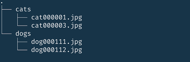
To use the ImageDataGenerator, you must structure your data a certain way on disk. For each label or category that you want to recognize, you have to create a subdirectory with the same name as the label. In that directory, you place the images of that specific category.

Distributing the training images

We have to copy the images from the zip from Kaggle into the directory structure, as discussed before. Also, to get an indication of how good our model is, we split the training images we got from Kaggle into a training and validation set. For example, we reserve 5,000 photos from the 25,000 for validating the trained model.

The following Python function distributes the cat and dog images from the folder where you unpacked the zip with pictures from Kaggle. The process creates a structure that can directly be used by the ImageDataGenerator.

The function retrieves a single parameter called validation_size. The validation size is a number between 0.0 and 1.0, representing the validation set’s proportion in the split.

The function shuffles the list of image names before it copies them to the correct directory. With this directory structure, we can start using the ImageDataGenerator.

Preparing the ImageDataGenerator

We will use the flow_from_directory method from the ImageDataGenerator. This method creates an iterator that retrieves and returns images from the specified directory.

I use the rescale parameter when creating an instance to rescale the pixels of the image automatically. Instead of using RGB values that range from 0 to 255, we rescale them into a floating-point number from 0 to 1. This rescale makes it easier to train the deep learning model.

We use the following parameters with the flow_from_directory method:

• directory — The directory that contains the subdirectories with the categories.
• target_size — Each image must be of the same size before submitting it to the deep learning pipeline. The ImageDataGenerator can perform this on the fly.
• batch_size — We submit the images to the deep learning pipeline in batches. This sets the size of the individual batches.
• class_mode — A hint of the type of data we read. In our case, ‘binary’ to show that we will use two categories.

When we run the code, the flow_from_directory reports the number of images found in what categories. In our case, the training generator reports 20000 images, and the validation generator reports 5000 images.

As the ImageDataGenerator is ready we can start creating and training the Deep Learning model

Creating and training the Deep Learning Model

As we have prepared the data, we can now start constructing the deep learning model using TensorFlow. We add the layers using the Sequential instance.

Convolutional layers

We split the model into three major parts. First, there are three combinations of the Conv2D and MaxPool2D layers. These are called convolution layers. A Conv2D layer applies a filter to the original image to amplify certain features of the picture. The MaxPool2D layer reduces the size of the image and reduces the number of needed parameters needed. Reducing the size of the image will increase the speed of training the network.

The second and actual Deep Learning Network starts on row eight, where we flatten the array. We create a hidden Dense layer with 512 units and use Rectified Linear Unit (relu) as the activation function.

The last part is the output layer. This last layer on row ten has a single output neuron. The output neuron will contain a value from 0 to 1, where 0 stands for a cat and 1 for a dog.

Compiling the model

Before we can start with training, we have to compile the model using the compile method. Compiling configures the model for training.

I choose the Adam optimizer as this is an excellent default to start with. The loss function is binary_cross_entropy because we are training a classification model with two possible outputs. I want to report the accuracy during training; therefore, I added accuracy as a metric.

The second-row calls summary() on the model. Calling the summary method produces an overview of the layers and the number of parameters. This is a great way to validate if you created everything you intended to create.

What we recognize in the summary is the decrease of the image’s size through the various layers. The picture starts as a 150x150 image and gets reduced through the multiple layers to a 17x17 sized image before entering the Deep Neural Network.

Training the model

After we compiled the model, we can start training the model. We can start the training by calling the fit method on the model instance.

The first parameter is the iterator that we created by calling the flow_from_directory of the ImageDataGenerator for the training data. The second parameter is the iterator from the validation data.

The epoch parameter shows how many times the model will process the entire training set. Here, I want to process all 20.000 training images 50 times.

The steps_per_epoch show how many batches it should process before it finishes the epoch. We established a batch size of 200 previously on the flow_from_directory, which gives 200 * 100 = 20,000 — the number of images of our training set.

The same goes for the validation_steps, 50 * 100 = 5,000, the number of images in our validation set.

During training, the fit method prints various metrics. Below you see that the accuracy on our training set at the end of the training is 0.99. The accuracy on the validation set is 0.79.

The model.fit method returns a history object which contains all the training data once the training is finished. This history object can be used to visualize the metrics.

Visualizing the training result

We can use the history object in combination with the Matplotlib library to visualize the loss and accuracy per epoch. The function below creates two graphs, one that shows the training and validation accuracy, and another that shows the training and validation loss.

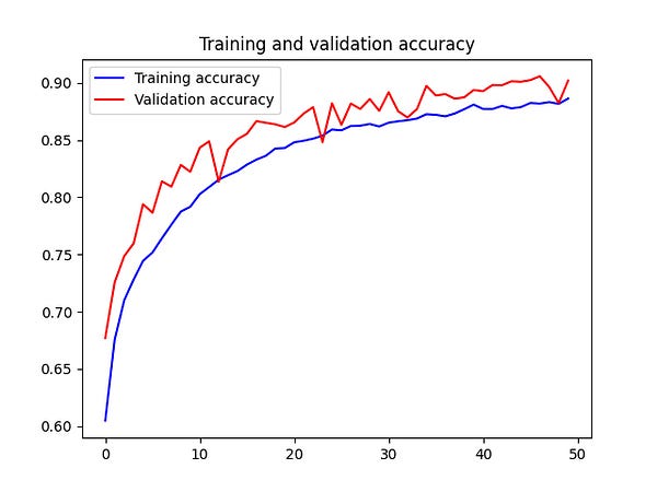
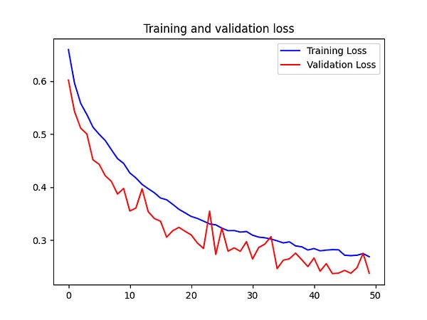
The plot_result function shows the following two graphs if you train the model for 50 epochs.

The interesting part is that the training set’s accuracy slowly increases to almost 1 (100%). However, the accuracy on the validation set increases to around 0.8 within the first five epochs and then flatlines at 0.8. This is the same for the loss of the validation set. It decreases the first four epochs and then increases again.

This is an obvious case of overfitting. The accuracy of the training set increases, but it can’t be generalized, clearly visible by the stagnation of the validation set’s accuracy.

Overfitting

Overfitting occurs when the model learns the training data so well that it can only predict the images that are from the training set. If we feed it images that are not from the training set it performs poorly.

We can overcome overfitting by using more data in your training data set. Here, this is difficult as we don’t have more images of cats and dogs from Kaggle. Luckily for us, there are other possibilities.

Optimizing the model

Before I create and submit a prediction to Kaggle, I want to see if we can optimize the model.

Image Augmentation

We saw that the accuracy on the validation set flatlined during training. We also discussed that you could improve the accuracy by increasing the amount of training data.

Instead of adding more training data, we could also use Image Augmentation. Image augmentation is a technique to create new artificial training data from the existing data. Image Augmentation changes the original training image by scaling, rotating, cropping, and flipping it. It artificially creates images for training.

The ImageDataGenerator we use can augment the images in memory once it loads them from disk. We can set the image augmentation options when we instantiate the ImageDataGenerator.

Previously we already used the ImageDataGenerator to rescale the images from disk. Now, we add additional options to augment the images.

We instruct the ImageDataGenerator to rotate, shift, zoom, flip, and shear within specific ranges. The ImageDataGenerator performs the augmentation at random. If we again train the model for 50 epochs using the ImageDataGenerator, we see the following accuracy and loss graphs.

Looking at the left graph that shows the validation accuracy, we see that it does not stop at 80% as we saw with the previous training. Instead, it climbs slowly to an accuracy of 90%.

The right graph shows the loss for both the training and validation set. Here we also see that they slowly and steadily decrease.

A much better result!

Creating a prediction

Before going further with optimizing the model, which is something for another article, we should upload our predictions of the test set to Kaggle to see how our model scores. After I trained the model, I saved it using the save method on the model.

In the load_and_predict method, we first load the model, then create a new ImageDataGenerator to serve the images from the test set to the model. We then call the predict method on the model to create the predictions from the test set.

The submission to Kaggle must be in a CSV format. We use Pandas to create a DataFrame from the predictions array. This DataFrame is saved to a CSV file and uploaded to Kaggle. Each submission is scored using the following log loss function.

My submission from the model using the CNN and Image Augmentation scored 0.26211. This would have put me around 833rd place on the public leaderboard.

This is a good start but I want to see I can improve the accuracy even further. But this is something for another article.

Conclusion

In this article, I described how to create and use a Convolution Neural Network using TensorFlow. This Neural Network was used to recognize Cats and Dogs from images. The images of the cats and dogs were taken from this old Kaggle competition Cats vs Dogs.

Although the competition is not running anymore, you can still upload and score your predictions of the test set. My CNN got a score of 0.26211 which got us on place 833rd place on the public leaderboard.

In an upcoming article, I will describe how we can further increase the accuracy using transfer learning.

The source-code for this article can be found on GitHub. The repository is pretty large as it includes all the training and test images.

Thank you for reading!