How to Simulate the Micromouse Competition With Python

A few days ago, I stumbled upon a fascinating YouTube video titled “The Fastest Maze-Solving Competition On Earth.” This documentary provides an inside look into the world of Micromouse competitions.

Micromouse events, unique in their character, pit miniature autonomous robots, aptly named ‘micromice’, against each other in a race through a maze. The mission is simple yet riveting: the quickest micromouse to find the exit triumphs.

The dimensions of the Micromouse play a crucial role. The micromouse robot must be at most 25 centimeters in length or width, even if its geometry changes during the competition.

While there are no restrictions on the robot’s height, it’s important to remember that a smaller size could be an advantage in navigating narrow paths within the maze.

As a technology enthusiast, the autonomous, intelligent operation of these micromice navigating through mazes to seek an exit was an exciting spectacle. The documentary thoroughly retrospects the competition’s history and highlights pivotal advancements that have propelled these maze-solving prodigies to greater speeds.

Among these breakthroughs, one ingenious solution stood out: a strategic counter to the micro mouse’s propensity to slip on the track.

Acknowledging that this was a factor shaving valuable time off their speed, the innovators came up with the idea to install a fan at the base of the mouse. This modification anchored the micromouse to the track, minimizing slippage and dramatically boosting its speed in navigating the maze.

Now, let’s paint a thrilling picture. Imagine bringing the adrenaline rush of the Micromouse competition to the digital arena. Visualize scripting your micromouse using Python, uploading it into a virtual game, and then watch it dash through a maze with lightning speed. Fascinating.

In this article, we’re poised to transform this vision into reality. We’ll create a digital version of the Micromouse competition and breathe life into a micromice.

All the coding examples this article covers are available for exploration and modification. You can find them in this dedicated GitHub repository.

Table of contents

· Physical to Digital: Navigating New Mazes
· Understanding the Micromouse Competition Rules
∘ Exploration phase
∘ Speed run phase
· Creating a Virtual Maze: Python’s Pathway to Puzzles
∘ Initialization
∘ Carving the maze
∘ Maze navigation
∘ Maze visualization
· A base for our virtual micromouse
∘ Inspect surroundings
∘ Moving
∘ Saving and loading exploration data
· Our first micro mouse, BasicMouse
∘ Exploring phase
∘ Speed run phase
∘ Loading the exploration data
∘ Finding the shortest path
· Running the Simulation
∘ Maze and Mouse Setup
∘ Event Loop Setup and Simulation Start
∘ Command-line Arguments
· Building Your Own Virtual Mouse
∘ Step and Move Methods
∘ Enhancing Your Mouse
· Conclusion

Physical to Digital: Navigating New Mazes

As we transition from physical mazes to digital ones, it’s worth exploring the benefits this shift brings to the table. By trading tangible labyrinths for virtual ones, we open a world of possibilities that weren’t feasible or cost-effective in the traditional Micromouse competition.

One of the main advantages of going digital is the ability to experiment with various algorithms rapidly. Physical micromice requires substantial time, effort, and resources to build, test, and modify. On the other hand, digital micromice can be iterated swiftly and conveniently within a software environment. This makes evaluating different navigation strategies and algorithms easier in real-time, enabling us to fine-tune our virtual micromouse to boost its maze-solving performance continually.

Furthermore, the digital realm allows us to test scenarios that may be impractical or impossible to replicate in a physical maze. We can introduce unexpected twists and turns, varying difficulty levels, and even dynamically changing mazes to challenge our micromouse in ways physical mazes can’t.

The most exciting advantage of digitizing the Micromouse competition is the opportunity to integrate machine learning into our navigation algorithms. Machine learning models can learn to identify the optimal path to the exit based on patterns and experiences. In the physical world, employing machine learning could be complex and expensive, requiring many sensors and a significant amount of time for data collection. In contrast, the digital world provides a controlled environment where machine learning models can be trained, validated, and fine-tuned more efficiently without the overhead of building and tweaking a physical robot.

The shift from physical to digital mazes represents an evolution of the Micromouse competition and an opportunity to expand our horizons in algorithmic problem-solving and artificial intelligence. We can transform these digital mazes into a thrilling sandbox for innovation and discovery by wielding Python as our tool.

Understanding the Micromouse Competition Rules

Navigating the twists and turns of the Micromouse competition requires more than just swift and smart mice; understanding the game's rules is equally crucial. Let’s break down the main guidelines that dictate how the competition unfolds:

A typical Micromouse competition is usually divided into two distinct phases.

Exploration phase

The first phase, the exploration phase, is where each micromouse can explore the maze. The micromouse starts at a designated corner of the maze and is given a certain time limit — usually around three minutes — to scout the labyrinth.

The goal during this phase is not to find the exit as quickly as possible but to map out the maze, record its intricacies, and identify the optimal path to the finish line. In this phase, speed takes a backseat to thoroughness and strategic planning.

The mouse records all this information for the second phase, the speed run.

Speed run phase

Once the exploration phase is over, the micromouse proceeds to the second phase: the speed run. During this phase, the micromouse leverages the information gathered in the exploration phase to navigate its way to the exit as swiftly as possible. The aim here is simple — reach the finish line in the least amount of time.

While the basic premise of the competition is straightforward, there are typically additional rules that micromice and their creators must adhere to, including size restrictions for the micromice and specific dimensions for the maze itself. However, these may vary between different competitions.

By adhering to these guidelines, participants can ensure a fair and exciting competition. It’s a delicate balance of exploration, speed, strategy, and algorithmic efficiency, turning each race into a riveting spectacle of technology and ingenuity.

It’s important to underscore the heart of the Micromouse competition: the remarkable display of intelligence embedded within these miniature robots.

Each micromouse is more than just a physical entity; it’s a testament to human innovation and ingenuity. Every line of code, every algorithm implemented, and every strategic decision is crafted by the creators and imbued into this tiny, autonomous creature.

Behind the scenes, the creators devote countless hours to building, programming, and refining these micromice, infusing them with the intelligence needed to conquer the maze.

The brilliance of their work is brought to life as these micromice navigate the labyrinth, revealing the beauty of technology and the power of well-applied logic. This blend of hardware and software, the physical and the digital, truly sets the Micromouse competition apart as a beacon of technological achievement.

Creating a Virtual Maze: Python’s Pathway to Puzzles

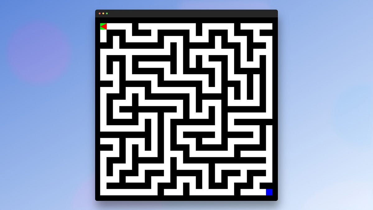
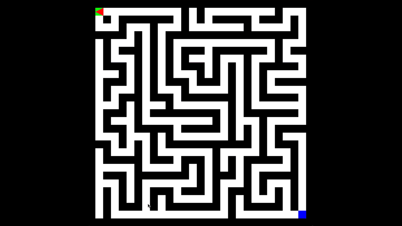
Our first step in devising this simulation is to construct a digital maze. The maze in our virtual domain echoes its physical counterpart, representing a 2D grid replete with walls, passages, and defined start and endpoints.

We’ll leverage an efficient maze generation algorithm — the Recursive Backtracker- to avoid the monotony and restrictions of manual maze creation. This ingenious tool enables the automatic fabrication of an intricate, comprehensive maze.

Another essential stipulation is regenerating an identical maze across multiple runs. This ensures the exploration and run phases of our Micromouse simulation consistently interact with the exact same maze, maintaining the integrity of our experiment.

The Maze class lies at the heart of our Python application, offering functionalities to create, navigate, and visualize a digital maze.

Below, I'm breaking down this class's critical components and methods to provide a better understanding.

Initialization

When an instance of the Maze class is instantiated, the __init__ method accepts four parameters - size, start, end, and seed. size determines the dimensions of the maze, start and end establish the maze's entry and exit points.

At the same time, seed initializes the random generator, allowing us to recreate identical mazes if needed. The self.cells list and self.visited_cells set tracks the cells and the cells visited in the maze.

class Maze: 
    def __init__(self, size, start, end, seed=0): 
        self.cells = [] 
        self.visited_cells = set() 
        self.size = size 
        self.start = start 
        self.end = end 
        self.grid = self._create_empty_grid() 
        self._create_cells() 
        random.seed(seed)  # set the random seed

Carving the maze

The generation of a valid path from the start to the endpoint in the Maze class is achieved using the carve_maze method. This method employs a depth-first search algorithm to carve a path, beginning from a specific cell (default or specified), and it keeps moving until all potential directions have been explored.

def carve_maze(self, current_cell=(1, 1)): 
    directions = [(0, 1), (0, -1), (1, 0), (-1, 0)] 
    random.shuffle(directions) 
    for direction in directions: 
        next_cell = (current_cell[0] + direction[0]*2, 
                     current_cell[1] + direction[1]*2) 
        if self._valid_next_cell(next_cell): 
            self._carve_path(current_cell, next_cell, direction) 
            self.carve_maze(next_cell)

Here’s a breakdown of how the carve_maze method ensures a valid path:

1. Starting from the current cell, the carve_maze function considers all possible directions (up, down, left, and right).
2. The order in which these directions are considered is randomized by shuffling the directions list. This step ensures that different runs of the function generate different mazes.
3. For each direction, the function calculates the position of the next cell by moving two units in the chosen direction.
4. The function then checks if this calculated next cell is a valid choice for carving a path using the _valid_next_cell function. A next cell is considered valid if it lies within the boundaries of the maze and is currently a wall (i.e., its value in the grid is 1). Remember that when starting, our Maze is filled with walls.
5. If the next cell is valid, a path is carved from the current cell to the next cell using the _carve_path function. This function changes the value of the cells from the current cell to the next cell in the chosen direction from wall (1) to passage (0).
6. The function then recursively calls itself, with the new cell as the current cell, ensuring a continuous path is carved.
7. If all directions from a cell have been explored (i.e., no valid next cells), the function returns and the path continues to be carved from the last cell in the recursion.

This recursive, depth-first approach guarantees that a continuous path is carved from the starting cell to some end cell.

Maze navigation

The get method retrieves the status of a specific cell in the maze. The add_to_visited_cells method marks a cell as visited during the exploration phase.

def get(self, row, column): 
    return self.grid[row][column] 
 
def add_to_visited_cells(self, position): 
    self.visited_cells.add(position)

Maze visualization

The draw method visually represents the maze using the Pygame library. It assigns colors to the start, end, walls, visited and unvisited cells. The specific color assignment is controlled by the _color_for_cell method.

def draw(self, screen): 
    for row in range(self.size): 
        for column in range(self.size): 
            cell_color = self._color_for_cell(row, column) 
            pygame.draw.rect(screen, cell_color, self.cells[row][column]) 
 
    pygame.draw.rect(screen, MicroMouseColor.GREEN, 
                     self.cells[self.start[0]][self.start[1]]) 
    pygame.draw.rect(screen, MicroMouseColor.BLUE, 
                     self.cells[self.end[0]][self.end[1]]) 
 
def _color_for_cell(self, row, column): 
    if self.get(row, column) == 1:  # wall cell 
        return MicroMouseColor.BLACK 
    elif (row, column) in self.visited_cells:  # visited cell 
        return MicroMouseColor.LIGHT_RED 
    else:  # unvisited cell 
        return MicroMouseColor.WHITE

A base for our virtual micromouse

In our architectural design, we’ve introduced a BaseMouse class. Every digital micromouse must inherit from this class, which provides essential methods that facilitate exploration of the maze environment.

Crucially, we aim to simulate realistic constraints faced by a physical micromouse. For instance, we do not want our digital mouse to have an omnipotent view of the entire maze. To implement this limitation, we’ve created a method named inspect_surroundings.

Inspect surroundings

Inspect_surroundings acts like a virtual sensor, providing information about the environment immediately adjacent to the mouse's current position. For each neighboring cell, it determines whether it's a wall or a passage.

This method serves as the micro mouse’s primary sensory tool. It’s the only way for a mouse subclassing from BaseMouse to gather information about its surroundings. The intelligence of navigating through the maze, therefore, depends on how effectively a mouse uses the information provided by this method.

def inspect_surroundings(self): 
    surroundings = {} 
    for direction, (dx, dy) in BaseMouse.MOVES.items(): 
        x, y = (self.position[0] + dx * self.view_distance, 
                self.position[1] + dy * self.view_distance) 
 
        if 0 <= x < self.maze.size and 0 <= y < self.maze.size: 
            surroundings[direction] = self._inspect_cell(x, y) 
 
    return surroundings

Moving

The BaseMouse class houses two pivotal methods for movement, namely step’ and move.

The step method, invoked by the game or event loop, is triggered each time an event associated with the mouse occurs. Within this method, the mouse must employ its sensory capabilities, inspecting its immediate surroundings to discern its next move.

Meanwhile, the move method alters the mouse’s actual position within the maze. This crucial transition process, however, is not implemented directly within the BaseMouse class.

The step method is the strategic core, making informed decisions based on environmental observations. In contrast, the ‘move’ method acts on these decisions, changing the mouse’s location within the maze.

The derived mouse should implement both these methods.

def move(self, direction): 
    raise NotImplementedError 
 
def step(self): 
    raise NotImplementedError

Saving and loading exploration data

The BaseMouse also contains the following helper methods to be able to load and save the data that has been gathered during the exploration phase.

def save_exploration_data(self): 
      data = self._prepare_exploration_data() 
      with open(self.exploration_data_location, 'w') as f: 
          json.dump(data, f) 
 
def load_exploration_data(self): 
    with open(self.exploration_data_location, 'r') as f: 
        data = json.load(f) 
    self._update_mouse_data(data) 
 
def _prepare_exploration_data(self): 
    return { 
        'visited': list(self.visited), 
        'walls': list(self.walls), 
        'maze_size': self.maze.size, 
        'goal': self.goal, 
        'start': self.start_position 
    }

1. save_exploration_data(self): This method saves the data gathered during the exploration phase of the micromouse. The data includes details about the visited cells, the walls, the maze's size, and the start and goal positions. This data is prepared by the _prepare_exploration_data method, converted into JSON format, and then written to a file specified by self.exploration_data_location. This method is typically called at the end of the exploration phase.
2. load_exploration_data(self): This method loads the data that was saved during the exploration phase. The data is read from a file specified by self.exploration_data_location, parsed from JSON format, and then used to update the state of the micromouse via the _update_mouse_data method. This method is typically called at the start of the run phase.
3. _prepare_exploration_data(self): This helper method is responsible for packaging up the data that needs to be saved at the end of the exploration phase. It creates a dictionary containing lists of the cells visited by the mouse and the walls discovered, along with the size of the maze and the start and goal positions.

These methods are essential to creating a realistic simulation of a Micromouse competition.

During a real competition, a micromouse first explores the maze to learn about its structure (the exploration phase). Then it uses this knowledge to find the quickest path from the start to the goal (the run phase). We can simulate this two-phase approach by saving the exploration data at the end of the exploration phase and then loading it at the start of the run phase.

Our first micro mouse, BasicMouse

Now it is time for our first digital micro mouse, BasicMouse. Remember that the mouse should support the exploring and speed run phases. We will start looking at the implementation of the exploration phase.

Exploring phase

In our MicroMouse simulation, the BasicMouse class extends from the BaseMouse class and implements an exploration phase using a common maze traversal technique called Depth-First Search (DFS).

Here is how the exploration phase works in the BasicMouse:

1. Step: In the step method, the mouse first checks if it has reached the goal using the at_goal method. If it has, it will stop. If not, it will initiate the explore method to search the maze.

def step(self): 
    if self.at_goal(): 
        return 
 
    self.explore() if self.is_exploring else self.follow_shortest_path()

2. Explore: The mouse's current position is marked as visited inside the explore method. The mouse then calls the inspect_surroundings method, which provides information about its immediate surroundings (north, south, east, and west).

def explore(self): 
    self.visited.add(self.position) 
    surroundings = self.inspect_surroundings() 
    unvisited_directions = self.get_unvisited_directions(surroundings) 
 
    if unvisited_directions: 
        self.move_to_unvisited(unvisited_directions) 
    elif self.stack: 
        self.backtrack()

3. Get Unvisited Directions: Using the get_unvisited_directions method, the mouse identifies the directions leading to open and not yet visited cells. It does this by iterating over the surroundings and filtering for passages (cell == 0) that have yet to be visited. If a cell is a wall (cell == 1), its position is added to the walls set.

def get_unvisited_directions(self, surroundings): 
    unvisited_directions = [] 
 
    for direction, cell in surroundings.items(): 
        new_position = self.add_direction_to_position(self.position, 
                                                      BaseMouse.MOVES[direction]) 
 
        # Only consider directions leading to open spaces and not previously visited 
        if cell == 1:  # if cell is a wall 
            self.walls.add(new_position) 
        if cell == 0 and new_position not in self.visited: 
            unvisited_directions.append(BaseMouse.MOVES[direction]) 
 
    return unvisited_directions

4. Move to Unvisited: If there are unvisited open passages, the mouse chooses one using the move_to_unvisited method and moves to that cell. It then marks this new position as visited.

5. Backtrack: If there are no unvisited open passages in the current cell and the stack of visited positions is not empty, the mouse will backtrack to the previous cell using the backtrack method.

The mouse continues this process of stepping, exploring, identifying unvisited directions, moving to unvisited cells, and backtracking until it reaches the end of the maze or has visited every reachable cell.

Upon reaching the goal, the mouse stops, marking the end of the exploration phase. The mouse now has a map of all the paths it has traversed, which can then be used in the run phase to identify the shortest route to the goal.

Speed run phase

The transition between the exploration phase and the speed-run phase in our program is controlled through command-line arguments. We designed it to provide a flexible interface that lets you easily switch between the two phases.

There are two main command-line arguments you can pass to the program. The first one is the seed argument. This lets you specify a seed for the random number generator, ensuring that the program generates the same maze on each run.

The second command-line argument is exploring. If you include this argument, the program will start in the exploration phase. Omitting it defaults the program to the speed-run phase.

Here’s how you would launch the program with a specific seed and initiate the exploration phase:

python ./app/main.py --seed 767 --exploring

In this command, --seed 767 sets the seed for the maze generation, and --exploring triggers the exploration phase. If you're ready for the speed-run phase, omit the --exploring flag.

Loading the exploration data

In the initial phase of our application, an instance of BasicMouse is created. Depending on the phase we’re currently in — exploration or speed run — this instance performs various actions.

If not in the exploration phase, the BasicMouse instance retrieves the exploration data from the previously saved JSON file. It then applies Dijkstra’s algorithm to determine the shortest path, and finally, it reconstructs this optimal path through the maze.

Here’s how this code snippet looks:

data_location = f"./app/mouse_exploration/exploration_data_{seed}.json" 
 
# Instantiate the BasicMouse 
mouse = BasicMouse(start, end, maze, exploration_data_location=data_location, 
                   is_exploring=exploring) 
 
# If we're not exploring, load the exploration data, run Dijkstra's algorithm,  
# and reconstruct the shortest path. 
if not exploring: 
    mouse.load_exploration_data() 
    mouse.run_dijkstra() 
    mouse.reconstruct_path()

In this example, if we’re in the speed run phase (i.e., exploring is set to False), the BasicMouse instance loads the exploration data, runs Dijkstra's algorithm on this data to find the shortest route, and subsequently reconstructs this path.

Finding the shortest path

The BasicMouse class employs Dijkstra's algorithm to determine the shortest path from its current position to the goal. It executes this algorithm during startup, storing the shortest route for use as it navigates toward the end.

Let’s break down the crucial methods that facilitate this process:

1. run_dijkstra(): This method applies Dijkstra’s algorithm to find the shortest path. It uses a priority queue (heap) to keep track of the nodes with the shortest distances and a set (visited) to track the nodes it has already processed. If it reaches the goal position, the method breaks from the loop, as it has found the shortest path.

def run_dijkstra(self): 
    heap = [(0, self.position)] 
    self.distances[self.position] = 0 
    visited = set() 
 
    while heap: 
        dist, current = heapq.heappop(heap) 
 
        if self.is_visited_or_distance_changed(current, visited, dist): 
            continue 
 
        visited.add(current) 
 
        if current == self.goal:  # stop when the goal is found 
            break 
 
        self.update_distances_and_predecessors(heap, current)

2. is_visited_or_distance_changed(): This helper method checks if a node has been visited or its distance has changed. If either condition is true, the method returns true. Otherwise, it returns false.

def is_visited_or_distance_changed(self, current, visited, dist): 
    return current in visited or dist != self.distances[current]

3. update_distances_and_predecessors(): This method updates the distances and predecessors of the neighboring nodes of the current node. It inspects the surroundings of the current node, calculates the new potential distance for each unvisited and not wall neighboring node, and updates the distance and predecessor if the new distance is shorter.

def update_distances_and_predecessors(self, heap, current): 
    surroundings = self.inspect_surroundings() 
    for direction, cell in surroundings.items(): 
        new_position = self.add_direction_to_position(current, 
                                                      BaseMouse.MOVES[direction]) 
 
        # only consider cells in the visited set and not walls 
        if self.is_valid_position(new_position): 
            self.update_distance_and_predecessor(heap, current, new_position)

With these methods, BasicMouse successfully applies Dijkstra's algorithm to determine the most efficient route to the maze's end, which it then utilizes for its journey.

Running the Simulation

To experience the virtual Micromouse in action, follow these simple steps. Here’s the gist of how our main application is structured to run the simulation:

The simulation program is initiated with the main function, which accepts a seed and an exploration flag as arguments.

Maze and Mouse Setup

First, we define parameters such as the maze size and the start and end points. We then initialize a Maze instance with these parameters and the provided seed, which helps control the randomness of the maze creation process. This is particularly useful if you want to rerun the same maze multiple times for testing different mice or strategies.

Afterward, we create an instance of our BasicMouse, supplying it with the maze, start and end coordinates, the location of the exploration data file, and a flag indicating whether we’re in exploration mode.

If we’re not in exploration mode, the mouse is instructed to load the exploration data from the previous run. It then utilizes Dijkstra’s algorithm to determine the shortest path from start to end based on the pre-recorded exploration data.

Event Loop Setup and Simulation Start

Subsequently, we initialize the MazeEventLoop, the main event loop responsible for handling user interactions and rendering the maze and mouse.

Finally, the simulation kicks off with a call to maze_event_loop.render_and_handle_events(). The maze is displayed, and the mouse starts its exploration or speed run, depending on the parameters provided.

Command-line Arguments

The simulation can be controlled via command-line arguments, allowing for convenient tweaking of the simulation parameters. If no arguments are provided, defaults are used. The --seed argument holds the random seed for the maze generation. The mouse will load exploration data at the start and execute its speed run by supplying the-- exploring flag. The mouse will start a fresh maze exploration if this flag is omitted.

For instance, to simulate exploration mode with a seed of 42, use

python ./app/main.py --seed 42 --exploring

Running the Micromouse simulation involves generating the maze, setting up the mouse, and letting the event loop handle the rest.

Building Your Virtual Mouse

Developing a virtual mouse to navigate our digital maze offers a unique opportunity to tackle problem-solving and algorithm design. All virtual mice must inherit from the BaseMouse class and implement the key methods, step, and move.

Step and Move Methods

The event loop calls the step method every time the mouse receives an action trigger. Here, the mouse should inspect its surroundings and determine its next move. The move method is where the mouse changes its position, effectively making the next move.

To start building your mouse, copy the BasicMouse class, rename it, and tweak its algorithms. The BasicMouse is a robust starting point, featuring Dijkstra's algorithm for shortest path calculation and a backtracking algorithm for maze exploration.

Enhancing Your Mouse

While the shortest path approach is efficient, other strategies can be adopted to improve the mouse’s performance during the exploration or speed run phase.

For example, one strategy could be to design the mouse to choose paths with the least number of turns instead of the absolute shortest distance. This approach might seem counterintuitive, but in real-life Micromouse competitions, maintaining a straight line and avoiding time-consuming turns is often quicker.

By inheriting from the BaseMouse class and customizing the mouse's exploration and pathfinding algorithms, you can craft a virtual mouse uniquely suited to tackle the maze.

Optimizing for fewer turns, faster execution time, or handling specific maze patterns, the possibilities are as vast as your imagination.

Remember, the objective is to get the mouse to the end of the maze and do so as efficiently and quickly as possible.

Enjoy the iterative design, testing, and optimization process — that’s where the real fun lies in the world of Micromouse!

Future Enhancements

While we’ve successfully implemented a robust and functioning virtual Micromouse environment, there’s always room for improvement and innovation.

Here are some prospective enhancements that would add extra depth and realism to the simulation and could form the basis for future projects or articles:

• Define Friction: To make the simulation more reflective of the real world, we could introduce the concept of friction. This would mean the mouse couldn’t instantly change its direction or speed, adding an extra challenge when writing mouse control algorithms.
• Account for Rotation Time: At the moment, our mouse can instantly turn without any time delay. Introducing a time cost for rotations would add another element to consider when creating efficient mouse algorithms, particularly in minimizing unnecessary turns.
• Enable Diagonal Moves: Currently, the mouse can only move in four cardinal directions: north, south, east, and west. Allowing for diagonal movements could open up a whole new range of strategies and paths to consider when programming the mouse.
• Create a Web Platform for Competition: We could develop a different web platform where users could upload their Micromouse scripts. This would not only allow them to test their code against a variety of different mazes but could also set the stage for virtual Micromouse competitions.
• Implement a Leaderboard System: To enhance the competition aspect further, we could implement a leaderboard system. This would track and display the top-performing mice across multiple runs or mazes, incentivizing participants to optimize their code.

These enhancements, while non-trivial, could significantly improve the complexity and realism of our virtual Micromouse environment. Whether you’re looking to refine your algorithm writing skills, build a web platform, or create a competitive coding challenge, there’s plenty to sink your teeth into.

Conclusion

In this journey, we’ve successfully developed a digital Micromouse simulation, designed and implemented a simple maze-exploring algorithm, and created a means for aspiring coders to build and test their virtual mice against our mazes.

This project demonstrates the powerful programming, algorithms, artificial intelligence, and even robotics applications in a fully virtual and accessible environment.

One of the key takeaways is the accessibility and versatility of this simulation. It can be an educational tool for those learning about AI or game theory, allowing enthusiasts to participate in the Micromouse challenge without needing physical hardware.

In terms of future improvements, there’s a wealth of possibilities. The scope for enhancement is vast, from refining the virtual environment with concepts such as friction and rotation time to implementing a web platform for a competitive coding challenge.

These improvements would add complexity and realism to the simulation, further enriching this project's educational and competitive aspects.

Finally, we’d love to see what you can do with the code. All the examples discussed in this article are available in this GitHub repository to explore, modify, and learn from.

We encourage you to take this code and make it your own, whether by tweaking the BaseMouse class or developing a whole new Micromouse algorithm from scratch.

This project offers an exciting and dynamic platform for learning and competition. We can’t wait to see what innovative solutions you’ll develop as we continue to improve and expand this virtual Micromouse environment together.

Happy coding!