Grip and Slip — Exploring F1 Tire Management With Python and Pandas AI
Python and Pandas AI illuminate the intricacies of F1 Racing
As the final echoes of the roaring engines faded into the night, Liam and Olivia, loyal Mercedes and Red Bull supporters, respectively, sat in contemplative silence.
The race was over, and Max Verstappen had claimed another victory. His Red Bull car, with its hard tires, glided across the finish line as though the track was its second home.
Liam broke the silence in his silver and turquoise Mercedes attire, leaning back and shaking his head in disbelief. “It’s the car,” he said, conviction ringing. “That Red Bull is just a beast on the track.”
Olivia, her cap bearing the charging Red Bull logo, was not so quick to attribute Verstappen’s success to his vehicle. She’d watched him, lap after lap, his times a marvel of consistency even on the hardest compounds.
“He’s the Tire Whisperer, Liam,” she countered, the nickname for Verstappen bringing a smile to her face. “There’s something in the way he drives… He knows how to make the tires last.”
The room lapsed into silence again, the two friends lost in their thoughts. Liam’s admiration for the craftsmanship of Mercedes and Olivia’s respect for the driver’s skill had often led them to these friendly debates. Still, a question was hanging in the air this time, a mystery waiting to be unraveled.
In the quiet aftermath of the race, an idea started to form in Olivia’s mind. “What if…” she began, turning to Liam with newfound excitement, “What if we could compare the lap times? Find out who is the most consistent driver?”
Liam looked at her, interest piqued. “You mean… use the lap data from the races? See who can make the most of their tires?”
Olivia nodded, her thoughts already spinning with the tantalizing possibilities. “Yes, exactly,” she responded. “Remember that Medium post I showed you about Pandas AI? It had this intriguing approach of interfacing with OpenAPI. We might be able to leverage that for this analysis rather than sticking to the method we used for the pit stops.”
Her eyes sparkled with excitement as she continued, “Of course, we’ll need to gather the data, scrub it clean, and dive deep into the analysis… but I have a hunch we can make it work.
It might even give us a new perspective on the drivers’ performance.
And so, beneath the dimming neon lights, their new investigation was born: a quest to uncover the secret of tire management in Formula 1 and find out who was the master of the race track.
All the source code, including the raw data, are available in this GitHub repository.
Finding the data
Olivia asked Liam to make her some coffee as she started to search to gather the data.
Coffee in hand, Olivia dove into her quest to collect the data. She needed to extract the lap times for all the drivers during the Miami Grand Prix, not forgetting to include the type of tire compound used by each one.
Lap times
“Where to begin?” she mused. Then it hit her. She’d used the Ergast REST API before, and it had exactly what she needed. The API included an endpoint that provided the lap times for each driver — perfect for her needs!
Eagerly, she navigated to the Ergast website, quickly finding the specific endpoint that held the key to her query. With a few swift keystrokes, she punched in the URL to pull up the lap times for the first lap of the Miami Grand Prix.
https://ergast.com/api/f1/2023/5/laps/1.json
Anticipation bubbled within her as she hit enter, and lo and behold, the screen blinked to life, revealing a neatly structured JSON response. See a part of it below.
{
 "Laps": [{
  "number": "1",
  "Timings": [{
   "driverId": "perez",
   "position": "1",
   "time": "1:36.191"
  }, {
   "driverId": "alonso",
   "position": "2",
   "time": "1:37.248"
  }, {
   "driverId": "sainz",
   "position": "3",
   "time": "1:38.078"
  }, {
   "driverId": "gasly",
   "position": "4",
   "time": "1:38.764"
  }]
 }]
}
Bingo! It was precisely what she was looking for — driver IDs, positions, and lap times. The only thing missing was the tire compound data. But she was not deterred; Olivia was just getting started and eager to tackle the next challenge head-on.
‘So far, so good,’ she thought, sipping her coffee and leaning back to admire the neatly laid out JSON data on her screen.”
Tire compound
Olivia scoured the Ergast API, hoping to find anything on the tire compounds. But to her dismay, there was nothing. “That’s odd,” she thought. “I’m sure I saw something about this in the Python Fast-F1 package…”
The Fast-F1 package had seemed like a neat little tool, wrapping up all the Ergast API information in a more user-friendly package. Yet it somehow provided more data than Ergast itself.
How could this be? Intrigued, Olivia delved into the source code. After all, the best thing about open-source software is that its secrets are there for anyone with the time and determination to find them.
After investigating, she found the answer and could not help but exclaim, “Aha!”
Liam, who’d been quietly sipping his coffee, looked up, startled. “What’s up?” he asked. Olivia grinned at him, “Next to the Ergast API, Fast-F1 also uses a different API — https://livetiming.formula1.com. That’s why it has more data.”
Liam’s eyebrows shot up in surprise. “Well, why don’t we use that one, too?” he asked. Olivia nodded slowly, “That’s a good idea, though I didn’t think this API was publicly available.”
She quickly pulled up a specific URL from the new API — https://livetiming.formula1.com/static/2023/2023-05-07_Miami_Grand_Prix/2023-05-07_Race/TimingAppData.jsonStream, which gave an exciting output.
01:07:40.985{"Lines":{"81":{"Stints":{"0":{"LapTime":"1:33.952","LapNumber":3}}}}}
01:07:42.047{"Lines":{"22":{"Stints":{"0":{"LapTime":"1:34.278","LapNumber":3}}}}}
01:07:42.579{"Lines":{"24":{"Stints":{"0":{"LapTime":"1:34.369","LapNumber":3}}}}}
01:07:43.063{"Lines":{"18":{"Stints":{"0":{"LapTime":"1:34.327","LapNumber":3}}}}}
01:07:43.985{"Lines":{"4":{"Stints":{"0":{"LapTime":"1:33.869","LapNumber":3}}}}}
01:07:45.266{"Lines":{"21":{"Stints":{"0":{"LapTime":"1:34.670","LapNumber":3}}}}}
01:07:49.985{"Lines":{"21":{"Stints":{"0":{"TotalLaps":3}}}}}
01:08:34.984{"Lines":{"2":{"Stints":{"1":{"TotalLaps":1}}}}}
01:08:45.015{"Lines":{"2":{"Stints":{"1":{"Compound":"MEDIUM"}}}}}
It was a sequence of timestamps followed by JSON data, packed with details of lap times and, crucially, tire compounds. Aha, there it was — the mention of the tire compound, just as she had hoped. ‘This number after ‘Lines’,’ Olivia pointed out to Liam, finger tracing the screen, ‘I believe that’s the driver number. This API has everything we need!’”
Reading the data
Okay, time to get down to brass tacks,” Olivia decided. It was clear to her that she would need to construct a few handy Python functions. Their task? Digest the data from the Ergast and Livetiming APIs and merge it into a comprehensive data structure encompassing all their necessities.
However, she noticed a slight hiccup in her plan. The rows in the live timing data utilized the drivers’ numbers to identify them, but the Ergast API used the driver IDs. “Looks like I’ll need a decoder ring,” she mused, resolving to construct a mapping system that would convert driver IDs from the Ergast API into the driver numbers used in the Livetiming data.
Then, an idea came to her. She could use ChatGPT’s web interface! Olivia found some relevant data on the internet and, using the capabilities of the AI, she converted it into a neat JSON file. This file would act as her ‘decoder ring’, helping her easily convert the IDs to numbers and vice versa.
“There we go,” she said with a satisfied nod, the JSON file open and ready on her screen. Now she was armed and prepared to tackle the data.
[
    {"id": "max_verstappen", "driver": "Max Verstappen", "team": "Red Bull", "number": 1},
    {"id": "sargeant", "driver": "Logan Sargeant", "team": "Wiliams", "number": 2},
    {"id": "norris", "driver": "Lando Norris", "team": "McLaren", "number": 4},
    {"id": "gasly", "driver": "Pierre Gasly", "team": "Alpine", "number": 10},
    {"id": "perez", "driver": "Sergio Perez", "team": "Red Bull", "number": 11},
    {"id": "alonso", "driver": "Fernando Alonso", "team": "Aston Martin", "number": 14},
    {"id": "leclerc", "driver": "Charles Leclerc", "team": "Ferrari", "number": 16},
    {"id": "stroll", "driver": "Lance Stroll", "team": "Aston Martin", "number": 18},
    {"id": "kevin_magnussen", "driver": "Kevin Magnussen", "team": "Haas", "number": 20},
    {"id": "de_vries", "driver": "Nyck de Vries", "team": "AlphaTauri", "number": 21},
    {"id": "tsunoda", "driver": "Yuki Tsunoda", "team": "AlphaTauri", "number": 22},
    {"id": "albon", "driver": "Alex Albon", "team": "Wiliams", "number": 23},
    {"id": "zhou", "driver": "Zhou Guanyu", "team": "Alfa Romeo", "number": 24},
    {"id": "hulkenberg", "driver": "Nico Hulkenberg", "team": "Haas", "number": 27},
    {"id": "ocon", "driver": "Esteban Ocon", "team": "Alpine", "number": 31},
    {"id": "hamilton", "driver": "Lewis Hamilton", "team": "Mercedes", "number": 44},
    {"id": "sainz", "driver": "Carlos Sainz", "team": "Ferrari", "number": 55},
    {"id": "russell", "driver": "George Russell", "team": "Mercedes", "number": 63},
    {"id": "bottas", "driver": "Valtteri Bottas", "team": "Alfa Romeo", "number": 77},
    {"id": "piastri", "driver": "Oscar Piastri", "team": "McLaren", "number": 81}
]
Parsing the lap times
Olivia decided to get the ball rolling with the Ergast API, diving headfirst into the lap times data. She created a dedicated class named LapTimeRetriever, which was tasked with doing just that — retrieving lap times.
At the heart of the LapTimeRetriever was the function process_lap_times. Olivia programmed it to meticulously request the lap times for all 57 laps of the Miami Grand Prix directly from the Ergast API.
def process_lap_timings(self, total_laps=57):
    all_lap_timings = []
    for lap_number in range(1, total_laps+1):
        lap_timings, from_cache = self.get_lap_timings(lap_number)
        all_lap_timings.append(lap_timings)
        if not from_cache:
            wait_time = random.uniform(2, 8)
            logger.info(f"Waiting for {wait_time} seconds before next request")
            time.sleep(wait_time)
    return all_lap_timings
Having set it all up, Olivia started running her code. However, Liam quickly noticed something off. “Oi, Liv. Why’s it taking an age to get through all the laps?” he queried, puzzled by the slow pace of the data retrieval.
Olivia, anticipating the question, explained her reasoning with a smile. “Well, Liam, it’s all about being considerate. After each request, I set up the program to pause for several seconds. This way, we don’t risk overloading the Ergast API.”
She paused for a moment, adding another layer to her answer. “Also, I’ve ensured we’re storing the data we retrieve locally. This means next time we run the program, we can pull the data from our disk instead of bombarding the API with repeated requests. It’s quicker and complies with the Terms and Conditions of the API.”
“Remember,” she concluded, grinning at Liam, “we’re getting all this valuable information for free. We ought to play nice.”
Deciphering tire compounds
“Hey Liam, you know this live timing API we’ve been working on, right? Well, it’s not exactly an open book. There’s no manual, no guide. But I’ve been picking it apart, trying to make sense of the info it holds about Formula 1 races.
Here’s what I’ve pieced together. Each chunk of data — let’s call it a JSON structure — starts with a timestamp. It’s probably recording the exact moment the data was collected, down to the millisecond.
Then, you’ll see something called ‘Lines.’ This looks like a key with many details about each car or driver attached. These details are linked to their racing numbers, which I’m guessing is what ‘RacingNumber’ means.
‘Stints’ is a term we are familiar with it. In our data, I think it’s referring to different parts of the race for each driver. At first, there’s not much under ‘Stints’, but it fills up with data as the race progresses.
Finally, ‘Compound.’ This is all about the tires. HARD, MEDIUM, SOFT — the type of tire compound they use.
But remember, Liam, I’m just interpreting from what I see — there’s no official word on this.
I’ve put together a class, the TireTypeRetriever, to make sense of it all. It reads, caches, and parses this live timing data. After much work, I managed to map it out in the following structure.
It starts with the driver’s number. Then it tells you what tire compound they began the race with and any changes they made during the race. Changes are marked with the lap number and the new tire compound.
{
 '1': [(1, 'HARD'), (46, 'MEDIUM')],
 '2': [(1, 'MEDIUM'), (3, 'HARD'), (4, 'MEDIUM'), (6, 'HARD')],
 '4': [(1, 'SOFT'), (5, 'HARD')],
 '10': [(1, 'MEDIUM'), (16, 'HARD')],
 '11': [(1, 'MEDIUM'), (21, 'HARD')],
 '14': [(1, 'MEDIUM'), (25, 'HARD')],
 '16': [(1, 'MEDIUM'), (18, 'HARD')],
 '18': [(1, 'HARD'), (43, 'MEDIUM')],
 '20': [(1, 'MEDIUM'), (15, 'HARD')],
 '21': [(1, 'MEDIUM'), (16, 'HARD')],
 '22': [(1, 'HARD'), (37, 'MEDIUM')],
 '23': [(1, 'MEDIUM'), (23, 'HARD')],
 '24': [(1, 'HARD'), (32, 'MEDIUM')],
 '27': [(1, 'HARD'), (34, 'MEDIUM')],
 '31': [(1, 'HARD'), (40, 'MEDIUM')],
 '44': [(1, 'HARD'), (38, 'MEDIUM')],
 '55': [(1, 'MEDIUM'), (19, 'HARD')],
 '63': [(1, 'MEDIUM'), (18, 'HARD')],
 '77': [(1, 'MEDIUM'), (16, 'HARD')],
 '81': [(1, 'SOFT'), (6, 'HARD')]
}
Combining it all in a Pandas data frame
Alright, Liam, now we’ve got all these bits and pieces, and it’s time to make them work together. We will tie them into a neat package — a single Pandas data frame. That way, we can later leverage Pandas AI, our goal.
So here’s what I did. I built this new class, right? I called it RaceDataRetriever. This class is handy because it uses all the previous ones I’ve built — DriverRetriever, LapTimeRetriever, and TireTypeRetriever.
There’s a special method in the RaceDataRetriever class; I’ve named it create_timing_dataframe. This method does all the heavy lifting. It takes the three classes and the data structures they produce and rolls them into one comprehensive data frame.
def create_timing_dataframe(self):
    current_lap = 1
    for lap_time in self.lap_times:
        for timing in lap_time:
            driver_number = self.driver_retriever.get_driver_number(timing['driverId'])
            compound = self.tire_retriever.get_compound(driver_number, current_lap)
            timing['compound'] = compound
        current_lap += 1

    data_flat = [item for sublist in self.lap_times for item in sublist]

    df = pd.DataFrame(data_flat)
    df['lap_number'] = df.groupby('driverId').cumcount() + 1

    return df
This final data frame holds every last piece of data we were looking for. Let me show you the data frame so you understand better, Liam.”
driverId position      time compound  laptime_seconds  lap_number
0            perez        1  1:36.191   MEDIUM           96.191           1
1           alonso        2  1:37.248   MEDIUM           97.248           1
2            sainz        3  1:38.078   MEDIUM           98.078           1
3            gasly        4  1:38.764   MEDIUM           98.764           1
4          russell        5  1:39.467   MEDIUM           99.467           1
5          leclerc        6  1:40.402   MEDIUM          100.402           1
6  kevin_magnussen        7  1:40.860   MEDIUM          100.860           1
7           bottas        8  1:41.314   MEDIUM          101.314           1
8   max_verstappen        9  1:41.724     HARD          101.724           1
9             ocon       10  1:42.184     HARD          102.184           1
Exactly, Olivia! This is precisely what we need,” Liam exclaimed. But as he was about to propose the next step, Olivia playfully interrupted him.
“Wait, let me guess,” she chimed in, a grin on her face. “You’re about to ask if I can… put the lap times of Max Verstappen into a graph, right?”
Analyzing the lap times

With a flair for vivid visual storytelling, Olivia employed Seaborn, a formidable Python library for data visualization, to construct a vibrant line graph. The graph didn’t just track lap times; it was a panoramic narrative of Max Verstappen’s stunning 2023 Miami Grand Prix race.
def plot_lap_times_single(df):
  fig, ax = plt.subplots(figsize=(10, 6))

  # Plot the line
  ax.plot(df['lap_number'], df['laptime_seconds'], linestyle='-', color='blue',
          linewidth=2, zorder=1)

  # Plot the markers
  compound_colors = {'MEDIUM': 'yellow', 'HARD': 'white'}
  for compound in df['compound'].unique():
      compound_df = df[df['compound'] == compound]
      ax.scatter(compound_df['lap_number'], compound_df['laptime_seconds'], marker='o',
                 s=120, facecolor=compound_colors[compound], edgecolor='black',
                 alpha=1.0, label=compound, zorder=2)

  # Find and plot the fastest lap
  min_time_row = df.loc[df['laptime_seconds'].idxmin()]
  fastest_lap = ax.scatter(min_time_row['lap_number'], min_time_row['laptime_seconds'], marker='o',
                           s=120, facecolor='violet', edgecolor='blue', zorder=3)

  ax.xaxis.set_major_locator(ticker.MaxNLocator(integer=True))
  ax.yaxis.set_major_formatter(ticker.FuncFormatter(lambda x, pos: seconds_to_mmsssss(x)))

  ax.grid(True)

  ax.set_title('Max Verstappen - 2023 Miami Grand Prix')
  ax.set_xlabel('Lap')
  ax.set_ylabel('Lap Time')

  # Create a custom legend
  from matplotlib.lines import Line2D
  custom_lines = [Line2D([0], [0], marker='o', color='yellow', label='MEDIUM',
                         markersize=10, markerfacecolor='yellow', markeredgecolor='black'),
                  Line2D([0], [0], marker='o', color='white', label='HARD',
                         markersize=10, markerfacecolor='white', markeredgecolor='black'),
                  Line2D([0], [0], marker='o', color='violet', label='Fastest lap',
                         markersize=10, markerfacecolor='violet', markeredgecolor='black')]

  ax.legend(handles=custom_lines)

  plt.show()
Olivia transformed mere data points into a captivating saga by ingeniously incorporating tire compound information and prominently spotlighting Max’s quickest lap.
Liam’s exclamation echoed, “Wow, this is remarkable, Olivia!” His gaze was riveted to the screen, tracing the consistent blue line representing Max’s lap times. “This graph is more than just a visual; it’s a goldmine of insights. The transition between tire compounds, the glorious purple dot that’s the fastest lap, it’s all brilliantly mapped out.”
Then, pointing at the declining curve of the line graph, his excitement peaked. “And look here,” he gestured enthusiastically, “See how Max’s lap times decrease as the race progresses? It’s a clear sign of the car getting lighter with each lap. This is data speaking volumes, turning numbers into an intriguing narrative!” The pride in his voice was tangible as he appreciated Olivia’s deft handling of the data.

Liam cast a cautious glance in Olivia’s direction. “Now, this might be pushing it a bit,” he began, his voice infused with curiosity and hesitation, “but is it possible to overlay the lap times of two drivers on the same graph? Say, for example, we chose Sergio Perez and Max Verstappen?”
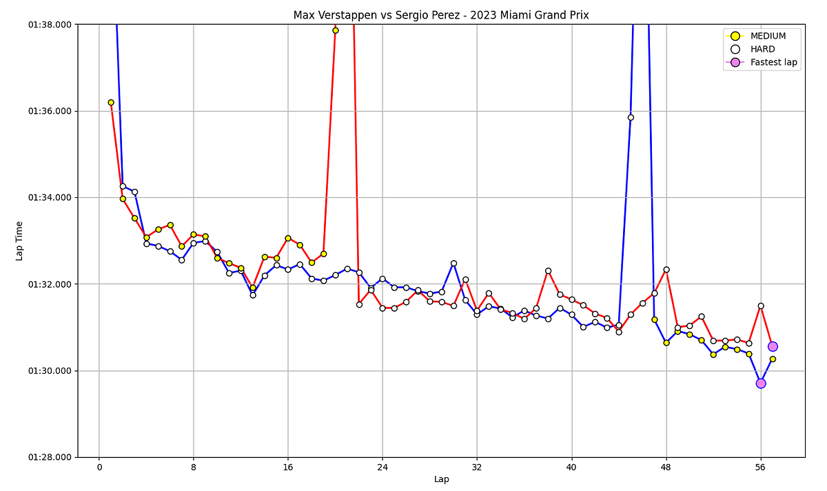
Olivia’s fingers barely hesitated above the keyboard. “Why not?” she said, a subtle smile creeping onto her lips. A series of keystrokes later, she adjusted the plotting function and restarted the application. As the screen refreshed, it unveiled an intriguing visual — a multi-dimensional graph that coalesced the lap times of Max Verstappen and Sergio Perez into one comprehensive visualization. An elegant blue line represented Max’s times, while a contrasting red line illustrated Sergio’s.
The room was filled with anticipatory silence as they studied the graph, the visual narrative of two racers unfolding before them.
Liam leaned closer to the screen, his eyes flitting across the distinct blue and red lines. “Incredible,” he breathed, awed by the story that the data was weaving.
“Look here, Sergio, with the advantage of starting up front, enjoyed clear air on the medium tires. However, even though Max started 9th on the harder compound, he still managed to clock faster lap times. And mind you, they both have identical cars.
His index finger traced the red line as it switched to reflect Sergio’s transition to the hard compound.
“You see, right after Sergio switched to the hard tires, he did clock a few faster laps,” he continued, “But here’s the real surprise — around the 40-lap mark, Max on his hard tires that were 40 laps old, began to outpace Sergio consistently. Now that’s truly impressive!”
The awe was unmistakable in his voice as he finished, echoing the wonder that the graph so vividly depicted.
Using Pandas AI
Excitement brimming in his voice, Liam turned to Olivia, “That was an impressive analysis, Olivia. Did you create that using that new tool — what was it, Pandas AI?”
Olivia shook her head, a modest smile tugging at the corners of her lips, “No, Liam, what we just worked on was pure Python using traditional pandas and Seaborn for visualization. As for Pandas AI, that’s a different beast altogether.”
Liam, clearly intrigued, followed up with another question, “Interesting. So, what do you envision doing with Pandas AI?”
Caught in thoughtful contemplation, Olivia eventually resumed, “Imagine, Liam, if we want to find the average lap time for Perez.
Instead of searching through the Pandas documentation to figure out how to achieve this, we could pose a direct question to our data frame in plain language via Pandas AI.
It’s like having a conversation with your data frame! Let me show you how this works in the code. You need an OpenAI API subscription to use Pandas.ai as it uses one of the OpenAI Large Language Models (LLM).
OPEN_API_KEY = os.environ.get('OPENAI_API_KEY')
llm = OpenAI(api_token=OPEN_API_KEY)
pandas_ai = PandasAI(llm)
result = pandas_ai.run(total_df, prompt='What is the average laptime of perez?')
print(result)
Olivia ran the code; moments later, the screen flashed with the operation results. Here’s what it displayed:
The average lap time of Perez is 92.34 seconds.Brimming with confidence, Olivia continued, “And we can go further. What if we want to know the average lap times for all drivers, not just Perez?” With a few more taps on the keyboard, she asked the query using pandas.ai.
result = pandas_ai.run(total_df, prompt='List all the average lap times of all drivers?')Just as before, the response flashed onto the terminal with remarkable speed. It presented a detailed list of drivers and their average lap times. Max Verstappen’s name stood out prominently, holding the fastest average lap time.
The average lap times of all drivers are as follows:
Albon with 93.53 seconds,
Alonso with 92.71 seconds,
Bottas with 93.51 seconds,
De Vries with 93.81 seconds,
Gasly with 93.23 seconds,
Hamilton with 93.15 seconds,
Hulkenberg with 93.56 seconds,
Kevin Magnussen with 93.35 seconds,
Leclerc with 93.18 seconds,
Max Verstappen with 92.25 seconds,
Norris with 93.79 seconds,
Ocon with 93.27 seconds,
Perez with 92.34 seconds,
Piastri with 94.26 seconds,
Russell with 92.83 seconds,
Sainz with 92.91 seconds,
Sargeant with 94.51 seconds,
Stroll with 93.39 seconds,
Tsunoda with 93.38 seconds, and
Zhou with 93.63 seconds.
Liam’s eyes lit up as he realized the possibilities. “This is incredible, Olivia,” he said, his voice filled with newfound excitement. “It feels like this tool is breaking down barriers. I may not be a data scientist, but I can dive into the data with Pandas AI and perform meaningful analysis!”
His words captured the exact potential of the AI-powered tool — to make data analysis approachable and accessible to everyone.
The Checkered Flag: Conclusions from our data race
Still excited, Liam turned to Olivia, his eyes sparkling with newfound understanding. “I’m starting to get the hang of this,” he announced with a grin. “And if I’ve got this right, there’s one more thing we need to do.” Olivia, arching an eyebrow, prompted him to continue.
“Well,” Liam said, his enthusiasm infectious, “it’s time we shared the fruits of your labor — this wonderful source code — with the community. We should ‘open source’ it, as you call it, right?”
Olivia responded with a laugh, nodding in agreement. “You’re spot on, Liam. I’m one step ahead of you, though. All the source code we’ve created, and the cached raw_data files for generating the graphs have been stored in a GitHub repository. It’s available for anyone to access and build upon.”
Liam excitedly turned to Olivia and proposed, “Let’s bring this all full circle and reflect on what we’ve discovered.”
They both reminisced about how the conversation had started. Max Verstappen’s victory of the 2023 Miami Grand Prix was initially thought to be all about having the best car, which Liam enthusiastically described as ‘a beast’. Olivia, however, offered a different perspective, arguing that it wasn’t just the car — Max was also a master at managing his tires.
Following that, Olivia showcased her data wizardry. “Remember how you found that data from all over the internet?” Liam asked, grinning. “Then you worked your magic, and we could visualize Max’s lap times with a line graph? It was like watching a story unfold right there in front of us. The story of Max Verstappen, the tire management maestro.”
The final piece of the puzzle was the introduction of Pandas AI. Liam’s eyes lit up as he remembered the moment. “That tool was a game-changer. It felt like you gave me the keys to a new world of data analysis. I could finally ask my own questions! How consistent are the lap times for my favorite drivers, Hamilton and Russel?”
“Exactly,” Olivia agreed, rising from her chair. “And now you have all the tools you need. Why don’t I get us a drink, and you can take the reins?” With a wink, she slid away from the keyboard, leaving Liam to explore the world of data analysis using Pandas AI, one question at a time.