Exploring Fractals With Python — Understanding the Beauty of Chaos

In the quest to understand the universe's complexities, humans have developed mathematical models and concepts that mirror its infinite variety and detail.

Among these, fractals hold a unique place. They present a fascinating confluence of math, science, and art, offering a key to understanding many of the intricate patterns that nature exhibits and being a source of aesthetically pleasing and infinite self-similar forms.

Fractals, coined by mathematician Benoit Mandelbrot in 1975, are derived from the Latin word ‘fractus,’ meaning broken or fractured. A fractal is a curve or geometric figure, each part having the same statistical character as the whole.

They are advantageous for modeling structures (such as eroded coastlines or snowflakes) in which similar patterns recur at progressively smaller scales and describing partly random or chaotic phenomena such as crystal growth, fluid turbulence, and galaxy formation.

The significance of fractals extends far beyond the realm of theoretical mathematics.

In nature, we encounter countless examples of fractal patterns. From the branching networks of rivers to the detailed structure of leaves and the spiral patterns of galaxies, the natural world tends to have fractal-like behavior.

The intricacy and self-similarity of fractals make them ideal for describing these complex phenomena with relatively simple mathematical expressions.

In the world of art, fractals have found a unique application. Their infinite complexity and inherently appealing patterns have led to their use in computer-generated imagery and design, creating stunning and captivating visual experiences.

Many artists and architects had unconsciously employed fractals long before the term was even coined, drawn by self-similar patterns' inherent beauty and harmony.

In essence, the study of fractals bridges the gap between the mathematical and the natural, the abstract and the concrete. This powerful concept extends its roots into multiple disciplines, paving the way for a deeper understanding of the intricate workings of the universe around us.

All the coding examples covered in this article are available for exploration and modification in the spirit of open collaboration and learning. You can find them in our dedicated GitHub repository.

Fractals and Python

Python emerges as a highly efficient tool for delving into the fascinating world of fractals, owing largely to its simplicity, versatility, and powerful libraries.

Its accessible syntax and readability make it especially useful for mathematical computations and visualizations — key aspects of exploring fractals.

Python houses many libraries that provide the requisite functionality for creating fractals.

For instance, NumPy, a powerful library in Python, is ideal for handling large, multi-dimensional arrays and matrices of numeric data. It offers a vast collection of mathematical functions to operate on these arrays, making it a great fractal tool.

Moreover, Matplotlib, another integral Python library, offers a comprehensive platform for creating static, animated, and interactive visualizations in Python. In fractals, this library is invaluable for visually representing these complex geometric structures, thus enabling a clearer understanding and appreciation of their infinite intricacy.

In essence, the combination of Python’s simplicity and the robust capabilities of its libraries, such as NumPy and Matplotlib, provides a powerful toolkit for diving into the captivating exploration and visualization of fractals.

Creating Basic Fractals with Python

Before diving into more complex fractals, we’ll start with two simpler ones: the Sierpinski Triangle and the Koch Snowflake. Both are classic fractal examples and are relatively easy to generate with Python.

The splendor of the Sierpinski Triangle

Named in honor of the esteemed Polish mathematician Waclaw Sierpinski, the Sierpinski Triangle is a captivating fractal pattern that emerges from the continual subdivision of a triangle into smaller triangles.

Sierpinski’s profound contributions to the world of fractal geometry are commemorated through several well-recognized fractals — the Sierpinski Triangle, the Sierpinski Carpet, and the Sierpinski Curve.

Delve into the essence of the Sierpinski Triangle with a Python function below. Leveraging the turtle module, this function iteratively generates Sierpinski Triangles, ascending from depth 1 to 6:

def draw_sierpinski(length, depth): 
    if depth == 0: 
        for _ in range(3): 
            turtle.forward(length) 
            turtle.left(120) 
    else: 
        draw_sierpinski(length / 2, depth - 1) 
        turtle.forward(length / 2) 
        draw_sierpinski(length / 2, depth - 1) 
        turtle.backward(length / 2) 
        turtle.right(60) 
        turtle.forward(length / 2) 
        turtle.left(60) 
        draw_sierpinski(length / 2, depth - 1) 
        turtle.right(60) 
        turtle.backward(length / 2) 
        turtle.left(60) 
 
def main(): 
    turtle.speed(0) 
    start_positions = [(-300, 200), (0, 200), (300, 200), 
                       (-300, -100), (0, -100), (300, -100)] 
    for depth, start_pos in zip(range(1, 7), start_positions): 
        turtle.penup() 
        turtle.goto(start_pos) 
        turtle.pendown() 
        start_time = time.time() 
        draw_sierpinski(150, depth) 
        end_time = time.time() 
        logger.info(f"Depth: {depth}, Took: {end_time - start_time:.2f}s") 
    turtle.hideturtle() 
    turtle.done() 
 
if __name__ == "__main__": 
    main()

Upon executing the script, the following visuals emerge, clearly showing the Sierpinski Triangles:

The Koch Snowflake: An Introduction

The Koch Snowflake, first introduced by the renowned Swedish mathematician Helge von Koch, is a seminal example of fractals. This form represents one of the initial fractal curves to be formally described.

The structure of the Koch Snowflake commences with a simple equilateral triangle, which is then iteratively transformed, with each line segment undergoing a recursive modification.

The Python function provided below utilizes the turtle module to illustrate the Koch Snowflake at ascending depths, ranging from 1 to 6:

def draw_koch(length, depth): 
    if depth == 0: 
        turtle.forward(length) 
    else: 
        draw_koch(length / 3, depth - 1) 
        turtle.left(60) 
        draw_koch(length / 3, depth - 1) 
        turtle.right(120) 
        draw_koch(length / 3, depth - 1) 
        turtle.left(60) 
        draw_koch(length / 3, depth - 1) 
 
def draw_koch_snowflake(length, depth): 
    for _ in range(3): 
        draw_koch(length, depth) 
        turtle.right(120) 
 
def main(): 
    turtle.speed(0) 
    starting_positions = [(x, y) 
                          for x in range(-200, 201) 
                          for y in range(200, -201, -200)] 
 
    for depth, pos in enumerate(starting_positions, 1): 
        turtle.penup() 
        turtle.goto(pos) 
        turtle.pendown() 
        start_time = time.time() 
        draw_koch_snowflake(100, depth) 
        end_time = time.time() 
        logger.info(f"Depth: {depth}, Took: {end_time - start_time:.2f}s") 
 
    turtle.done() 
 
if __name__ == "__main__": 
    main()

Executing this script will generate six Koch Snowflakes with an increasing depth from 1 to 6, as you can see below.

An intriguing aspect of fractals is the exponential increase in complexity with each increase in depth.

For instance, when generating a Koch snowflake, we begin with a single line segment at depth 0.Upon reaching depth 1, this distinct segment morphs into four. At depth 2, each of these four segments divides again, resulting in 16 elements. The process continues this way; by depth 6, we are confronted with more than 4,000 segments.

This exponential increase in drawing operations is primarily why the turtle module’s performance dwindles at greater depths. Simply put, the computational demand grows dramatically with each additional level of complexity.

The table below presents the time required to generate a snowflake at each depth, illuminating the escalating computational demand.”

Both these fractals, while simple, showcase the fundamental property of fractals: self-similarity across scales. Regardless of how much you zoom in, you will see the same shape repeated repeatedly. This property is one of the reasons why fractals are so fascinating and have numerous applications across different fields.

Exploring the Mandelbrot Set

The Mandelbrot set, a fascinating and iconic example of a fractal, is an intriguing study for anyone interested in fractals.

Named after its discoverer, the mathematician Benoit Mandelbrot, this set has a seemingly simple definition yet generates an infinitely intricate structure, reflecting the hallmark self-similarity characteristic of fractals.

The set’s captivating complexity and striking visualizations have made it a significant figure in mathematics and beyond.

The mathematical formula behind the Mandelbrot set is a deceptively simple iterative process. For a given complex number c, we start with a second complex number z, initially set to zero, and repeatedly apply the formula z = z² + c.

The number c is considered in the Mandelbrot set if applying this formula iteratively doesn’t send z off to infinity. Despite the simplicity of this rule, the resulting figures are infinitely complex and reveal an endless variety of shapes upon zooming in, showcasing the rich geometry of the set.

To visualize the Mandelbrot set using Python, one can follow these general steps:

1. Import the necessary libraries, namely NumPy for numeric computations and Matplotlib for plotting.
2. Define the resolution and boundaries of the plot in the complex plane.
3. For each point c in the complex plane, initialize z to zero and iteratively apply the formula z = z² + c. Track whether z stays bounded within a certain range through a predetermined number of iterations.
4. Use these results to assign a color to each point c, often using the number of iterations it took for z to escape to infinity. This step is where Matplotlib’s powerful visualization tools come into play.
5. Plot the results and marvel at the beautiful, infinitely complex figure that emerges.

def mandelbrot(c, max_iter): 
    z = c 
    for n in range(max_iter): 
        if abs(z) > 2: 
            return n 
        z = z*z + c 
    return max_iter 
 
def draw_mandelbrot(xmin, xmax, ymin, ymax, width, height, max_iter): 
    r1 = np.linspace(xmin, xmax, width) 
    r2 = np.linspace(ymin, ymax, height) 
    return (r1, r2, np.array([[mandelbrot(complex(r, i), max_iter) for r in r1] for i in r2])) 
 
def main(): 
    dpi = 80 
    img_width = dpi * 10 
    img_height = dpi * 10 
    xmin, xmax, ymin, ymax = -2.0, 1.0, -1.5, 1.5 
    max_iter = 256 
 
    x, y, z = draw_mandelbrot(xmin, xmax, ymin, ymax, img_width, img_height,  max_iter) 
 
    plt.figure(figsize=(img_width/dpi, img_height/dpi), dpi=dpi) 
    plt.xticks([]) 
    plt.yticks([]) 
    plt.title("Mandelbrot Set") 
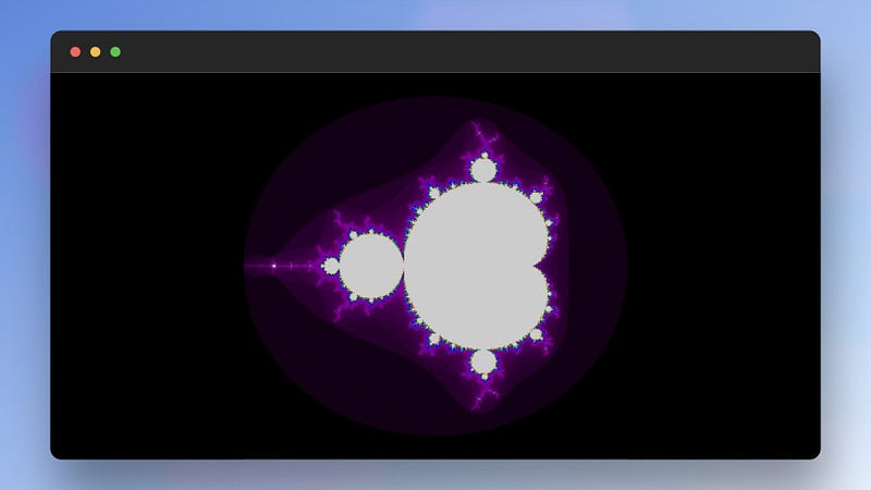
    plt.imshow(z, origin='lower', cmap='nipy_spectral') 
    plt.show() 
 
if __name__ == "__main__": 
    main()

This script generates the following mandelbrot.

A fascinating experiment to consider involves progressively zooming into the Mandelbrot figure using Python. By capturing and storing an image at each zoom level, we can amass a collection of .jpg files.

When assembled in sequence, these individual frames coalesce into a captivating movie, presenting a real-time journey into the depths of the Mandelbrot set.

Below is the Python script devised to generate each individual .jpg file. Feel free to explore and adjust parameters as you delve deeper into the intricacies of fractals.

def mandelbrot(c, max_iter): 
    z = c 
    for n in range(max_iter): 
        if abs(z) > 2: 
            return n 
        z = z*z + c 
    return max_iter 
 
def draw_mandelbrot(xmin, xmax, ymin, ymax, width, height, max_iter): 
    r1 = np.linspace(xmin, xmax, width) 
    r2 = np.linspace(ymin, ymax, height) 
    return (r1, r2, np.array([[mandelbrot(complex(r, i), max_iter) 
                               for r in r1] for i in r2])) 
 
img_width = 800 
img_height = 800 
max_iter = 256 
 
# Ensure the 'output' directory exists 
os.makedirs('output', exist_ok=True) 
 
for frame in range(50): 
    zoom = 0.05 * frame 
    xmin, xmax = -0.74877 + zoom, -0.74872 - zoom 
    ymin, ymax = 0.065053 + zoom, 0.065103 - zoom 
    dpi = 80 
    fig = plt.figure(frame, dpi=dpi, figsize=(img_width/dpi, img_height/dpi), 
                     frameon=False) 
    ax = plt.Axes(fig, [0., 0., 1., 1.], ) 
    ax.set_axis_off() 
    fig.add_axes(ax) 
    r1, r2, mandelbrot_image = draw_mandelbrot(xmin, xmax, ymin, ymax, img_width, 
                                               img_height, max_iter) 
    ticks = np.arange(0, img_width, 3*dpi) 
    x_ticks = r1[ticks] 
    plt.xticks(ticks, x_ticks) 
    y_ticks = r2[ticks] 
    plt.yticks(ticks, y_ticks) 
    ax.set_xticks([]) 
    ax.set_yticks([]) 
    ax.imshow(mandelbrot_image, origin='lower', cmap='nipy_spectral', extent=(xmin, xmax, 
                                                                              ymin, ymax)) 
    plt.savefig(f'./output/frame_{frame}.jpg') 
    plt.close()

Once all the individual .jpg files are saved in the output folder, we employ FFmpeg, a powerful multimedia framework, to stitch these frames together and create a fluid .mp4 animation. This process provides us with a dynamic and visually engaging exploration of the Mandelbrot set.

ffmpeg -f image2 -r 10 -i ./frame_%2d.jpg -vf reverse animated.mp4

I then converted the mp4 into a gif to show the animation in this article using this FFmpeg script from High qualify GIF with FFmpeg.

palette="/tmp/palette.png" 
filters="fps=15,scale=320:-1:flags=lanczos" 
 
ffmpeg -v warning -i $1 -vf "$filters,palettegen" -y $palette 
ffmpeg -v warning -i $1 -i $palette -lavfi "$filters [x]; [x][1:v] paletteuse" -y $2

Exploring the Julia Set

As we delve further into fractals, another captivating set awaits us: the Julia Set. Named after the French mathematician Gaston Julia, the Julia Set shares a deep-rooted connection with the Mandelbrot Set.

Where the Mandelbrot Set answers the question of stability for a quadratic function centered around zero and various complex constants, the Julia Set takes a specific complex constant. It investigates the behavior of every complex seed under iteration.

Unlike the Mandelbrot Set, which remains constant, each distinct choice of the complex constant gives us a different Julia Set. The variations in the constant parameters result in a wide variety of fractal images, each with its distinctive shape and character.

Here is a Python script to generate and visualize six different Julia sets:

def julia_set(c, xlim, ylim, res, max_iter): 
    x = np.linspace(xlim[0], xlim[1], res[0]) 
    y = np.linspace(ylim[0], ylim[1], res[1]) 
    X, Y = np.meshgrid(x, y) 
    img = np.zeros(X.shape, dtype=float) 
    Z = X + 1j * Y 
    for i in range(max_iter): 
        Z = Z**2 + c 
        mask = np.abs(Z) < 1000 
        img += mask 
    img = img / img.max() 
    return img 
 
def main(): 
    c_values = [-0.7, -0.8j, -0.7+0.3j, 0.27, -0.4+0.6j, 0.37-0.1j] 
 
    fig, axes = plt.subplots(2, 3, figsize=(12, 8)) 
 
    axes = axes.flatten() 
 
    for ax, c in zip(axes, c_values): 
        img = julia_set(c, xlim=(-1.5, 1.5), ylim=(-1.5, 1.5), 
                        res=(500, 500), max_iter=200) 
        ax.imshow(img, extent=(-1.5, 1.5, -1.5, 1.5), cmap='nipy_spectral') 
        ax.axis('off') 
        ax.set_facecolor('black') 
 
    fig.patch.set_facecolor('black') 
 
    plt.tight_layout() 
    plt.show() 
 
if __name__ == "__main__": 
    main()

This will generate the following figures.

Fractals in Nature and Real-World Applications

Fractals are not merely abstract mathematical constructs. They are also ubiquitous in the natural world. It’s remarkable how these self-similar structures generated by iterative processes can also be found in various natural phenomena.

For instance, fractal patterns are evident in the branching of trees or veins, the intricate design of snowflakes, the shape of coastlines, and even the distribution of galaxies in the universe.

The famous Romanesco broccoli is a perfect example of a natural fractal, where each bud is composed of smaller buds, all arranged in yet more logarithmic spirals.

Moreover, fractal studies have also found practical applications in various scientific and technological fields.

In computer graphics, fractal algorithms are utilized to create realistic landscapes, textures, and other complex patterns computationally efficiently.

This is because fractals can mimic the irregularity and complexity found in nature with relatively simple mathematical constructs.

In data compression, fractal techniques have been developed to compress image and video files to a fraction of their original size while maintaining a high level of detail upon decompression.

In studying chaotic systems — systems susceptible to initial conditions, like the weather — fractals help provide a mathematical framework for understanding and predicting such complex dynamics.

Despite their mathematical complexity, fractals, with their inherent self-similarity and infinite complexity, are a powerful tool for understanding the complexities of nature and the universe and solving real-world problems.

Conclusion

Fractals' self-similar patterns, infinite complexity, and captivating beauty intersect art and mathematics. These fascinating constructs, created through simple iterative processes, illustrate the profound idea that complexity can arise from simple rules.

The exploration of fractals in this article underscores their abstract mathematical beauty and ubiquitous presence in our natural world.

From tree branches to galaxies, these intricate patterns echo the inherent fractal designs found in nature, a testament to the universal language of mathematics.

Moreover, the practical implications of fractals extend far beyond their natural occurrences. They have permeated various scientific and technological fields, aiding in computer graphics, contributing to data compression techniques, and providing insights into chaotic systems.

But our journey into the world of fractals need not stop here. I encourage you to delve deeper, experiment with different fractal equations and parameters, and explore the captivating fractal universes that unfold.

Each new parameter is a new journey, and each fractal is a universe in its own right, waiting to be discovered.

With their blend of aesthetics and science, fractals truly embody the sentiment that there’s an undeniable beauty in complexity. We can perceive the intricate mathematical rhythms underlying our complex world through them.

All the coding examples covered in this article are available for exploration and modification in the spirit of open collaboration and learning. You can find them in our dedicated GitHub repository, which we continuously update with new and interesting explorations in fractal mathematics.

Happy coding!