AI in the Fast Lane: Predicting F1 With PyTorch

Olivia knocked on the door of Liam’s apartment, expecting to be greeted by his usual exuberant energy. However, she found him in a rather somber mood when the door creaked open. His living room walls, adorned with posters of iconic Ferraris, seemed to reflect his disappointment.

“Liam, you okay?” she asked, taking in his dejected expression.

He sighed deeply, “Sainz missed the podium in the last race. That, combined with my terrible prediction in the playing pool… I’ve dropped several places.” He motioned towards a leaderboard on his computer screen, showcasing his current rank in the Formula 1 sports prediction pool they both participated in.

Olivia sat beside him, trying to find words of comfort. “Races are unpredictable, and so are predictions. That’s the thrill of it, right?”

Liam let out a small chuckle, “You always know how to cheer me up. But still, I wish there was a way to make better predictions. It’s so difficult, especially this season.”

Olivia’s eyes lit up, sensing an opportunity, “What if we could bring some tech magic into this? Ever thought of using AI for your predictions?”

His curiosity piqued, Liam leaned in, eager to dive deep into this new challenge with Olivia. They were about to embark on a thrilling journey, merging their love for Formula 1 with the power of neural networks.

Note to Readers: For those interested in the technical aspects of our journey, the complete source code and a detailed walkthrough of our machine-learning model are available on GitHub.

You can explore the code, experiment with it, and contribute to its evolution. Visit the F1-predictor GitHub Repository to dive into the code that powers our predictions.

GitHub - PatrickKalkman/F1-predictor: A repository that contains all the examples that go with a…

A repository that contains all the examples that go with a Medium article about creating a deep neural network using…

Olivia paused momentarily, gathering her thoughts, then looked up at Liam with determination in her eyes. “Let’s be strategic about this,” she began. “Predicting the exact finishing order for all drivers in a race is a highly complex task, especially if we consider all the variables at play in a race.”

Liam nodded in agreement, recognizing the complexity of the task at hand.

Continuing with her thought, Olivia said, “Instead of spreading ourselves too thin, let’s first focus on predicting the outcome for a single driver. We can aim to determine whether this particular driver will finish 1st, 2nd, 3rd, and so on. Once we have a reliable model for one driver, we can expand our model to predict outcomes for other drivers or even the entire grid.”

Liam considered this approach momentarily before responding, “That sounds like a smart way to tackle it. Let’s first predict the race outcome for our chosen driver and build from there.”

“Exactly,” Olivia affirmed, feeling optimistic about the road ahead. “We’ll take it one step at a time and refine our model as we progress.”

Liam’s face lit up with realization, “Hey, remember when we looked into the decreasing pitstop times using that public API? The Ergast API! It has a ton of historical Formula One data. Maybe we could leverage that?”

How To Uncover the Secrets of F1 Pit Stops — A Python-Powered Analysis

Leveraging data analysis to unravel Formula 1 pit stop patterns

Olivia smiled approvingly, “Exactly! That’s a great starting point. Using the Ergast API, we can access vast historical data to feed our neural network. Let’s lay down a structured roadmap to cover all bases.”

She began outlining the process:

1. Data Collection:
Use the Ergast API to gather relevant historical F1 data.

2. Data Preprocessing:
Clean and normalize the data, ensuring it’s ready for the neural network.

3. Data Analysis:
Identify patterns, trends, and key features that influence race outcomes.

4. Neural Network Design:
Set up an appropriate architecture for the model.

5. Data Encoding:
Convert categorical data into a machine-readable format.

6. Dataset Management:
Divide the data into training, validation, and test sets.

7. Model Training & Evaluation:
Train the model using the training set, validate its performance, and test its accuracy.

8. Predictive Analysis:
Start with predicting the next race winner and gradually progress to predicting the top 10.

9. Model Refinement:
Iteratively fine-tune the model based on prediction feedback.

Data Collection & Preprocessing

“Alright, Liam, let’s get down to brass tacks,” Olivia began, eyes narrowing in concentration. “To build an effective deep learning model, we need a robust dataset — a treasure trove of features that could help us nail those F1 race predictions.”

Liam, pouring over Ergast's folders, said, “We’re in luck, Olivia. This Ergast export is a data enthusiast’s dream! Fourteen separate CSV files, each a deep well of information. The challenge is sifting through this mountain of data to find the gems that will make our model shine.”

With a knowing smile, Olivia replied, “Ah, the age-old problem of ‘feature selection.’ But that’s where our years as F1 fans pay off. Our familiarity with the sport gives us the domain expertise to identify crucial factors. The circuit characteristics, team dynamics, and drivers’ starting positions can be game-changers.”

Liam, visibly excited, took out a notepad. “So, let’s inventory what we’ve got. We’ve got a results.csv file that lists the outcomes of 26,000 races. There's a drivers.csv that profiles the various competitors. We also have constructors.csv for team details, qualifying.csv for initial race positions, and lastly, races.csv and circuits.csv that lay out the nitty-gritty of each race event and its venue."

Olivia nodded, her eyes gleaming with the thrill of the impending challenge. “Excellent, that gives us a lot to work with. Our first task is to harmonize these disparate files into one master dataset, intricately weaving each feature to create a tapestry of predictive power.”

“Time for some coding magic, don’t you think?” Olivia cracked her knuckles and opened her laptop. “I’ve got some Python functions to help us collate and process the CSV files. Python’s Pandas library is a lifesaver for this sort of data manipulation. It’s like Excel on steroids!”

Liam leaned in, eyes wide. “Lay it on me, code guru!”

The Data Loading Functions

1. load_csv Function

“First, I’ve got a function called load_csv. It reads any CSV file and can drop columns we don't need," Olivia explained as she opened her IDE.

def load_csv(file_path, drop_columns=None): 
    """Load CSV and optionally drop specified columns.""" 
    df = pd.read_csv(file_path) 
    if drop_columns: 
        df.drop(columns=drop_columns, inplace=True) 
    return df

Specialized Loading Functions

“Then, I’ve got specialized functions for each CSV we’ve got. Take the drivers, for instance. I load the CSV and keep only the columns we need. I even merge their first and last names into a full name.”

def load_drivers(): 
    """Load and process the drivers data.""" 
    drivers_df = load_csv('./data/drivers.csv', 
                          ['driverRef', 'number', 'code', 'dob', 'nationality', 'url']) 
    drivers_df['full_name'] = drivers_df['forename'] + ' ' + drivers_df['surname'] 
    drivers_df.drop(columns=['forename', 'surname'], inplace=True) 
    return drivers_df

She continued, showing off similar functions for circuits, races, constructors, qualifying, and results.

Merging DataFrames

“After that, I’ve got a neat little function that merges all these specialized DataFrames into one. It’s recursive and quite flexible.”

def merge_dataframes(base, *args, **kwargs): 
    """Recursively merge data frames.""" 
    if not args: 
        return base 
    return base.merge(merge_dataframes(*args), **kwargs)

The Master Function: load_and_process_data

“And finally, the pièce de résistance, load_and_process_data. This function combines it, invoking the specialized loaders, merging the data, and cleaning it up."

def load_and_process_data(): 
    """Load and preprocess the data.""" 
    drivers_df = load_drivers() 
    circuits_df = load_circuits() 
    races_df = load_races() 
    races_df = races_df.merge(circuits_df, on='circuitId').drop(columns=['circuitId']) 
    constructors_df = load_constructors() 
    qualifying_df = load_qualifying() 
    results_df = load_results() 
 
    # Data Merging 
    dfs_to_merge = [(qualifying_df, ['raceId', 'driverId']), (races_df, 'raceId'), 
                    (drivers_df, 'driverId'), (constructors_df, 'constructorId')] 
 
    for df, on in dfs_to_merge: 
        results_df = results_df.merge(df, on=on, how='left') 
 
    # Data Cleanup 
    cleanup_data(results_df) 
 
    return results_df

Liam sat back, genuinely impressed. “Olivia, you’re an artist with code. This is like painting but with functions and loops!” Olivia grinned, “Well, coding is more fun when you’re predicting Formula 1 races, don’t you think?”

Olivia swiveled her screen toward Liam and announced, ‘Feast your eyes on our ‘result’ DataFrame.’ The top five rows illuminated her display. ‘We’re working with 15,273 entries here.’

Liam’s eyes narrowed. ‘Wait, what happened to the other 10,000 entries?’

Olivia leaned back in her chair, ‘Great question. I pruned the rows where the ‘result’ column was empty, most likely indicating the driver didn’t finish the race — so, a DNF.’

Intrigued, Liam proposed, ‘That’s an interesting approach, but shouldn’t we consider including those DNFs and perhaps assigning them a result value of zero?’

Olivia pondered momentarily, ‘You’ve got a point there, Liam. However, let’s proceed with this pruned dataset and see how the model performs. We can always circle back and tweak.

Data Encoding

Eager to move forward, Liam exclaimed, ‘Alright, we’re all set! Let’s dive into the training phase.’

Olivia raised her hand, signaling him to slow down. ‘Hold your horses. We’re not quite there yet. Our data frame needs to transform to make it neural net-friendly.’

‘And what does that mean?’ Liam asked.

Olivia explained, ‘Essentially, neural networks function optimally with numerical data. So, categorical information, like the driver’s name, must be converted into numerical form.’

Liam scratched his head, ‘Alright, I get it. But how do we make that conversion?’"

Olivia leaned back in her chair, deep in thought. “There are multiple ways to encode categorical data for neural networks. One common approach is one-hot encoding, which turns each category into a unique array of zeros and ones.”

Liam furrowed his brow, “So, for example, if we have three drivers — let’s say Hamilton, Verstappen, and Sainz — Hamilton could be [1, 0, 0], Verstappen could be [0, 1, 0], and Sainz could be [0, 0, 1]?”

“Exactly,” Olivia affirmed, “and not just the drivers, but other categorical variables like circuits and constructors would also undergo the same transformation.”

“That makes sense. So, once everything is in numbers, our neural network will be able to make sense of it?” Liam asked, finally grasping the concept.

“Yes,” Olivia said with a smile. “Once all our data is numerical, we can then normalize it to ensure that all features have the same influence on the model. And then, my friend, we’ll be all set to train our neural network.”

Liam’s eyes lit up, “Ah, the light at the end of the tunnel! Let’s do this, Olivia.”

Olivia navigated back to her code editor, diving deeper into the next part of the data preprocessing. “We have three columns that need transformation: ‘circuit,’ ‘name,’ and ‘constructor.’

Instead of using pandas’ built-in function, I’m employing the OneHotEncoder from scikit-learn. It’s more efficient for large datasets and provides reusability, which is crucial for our predictions.”

Liam raised an eyebrow, curious. “Reusable? How does that work?”

With a knowing smile, Olivia explained, “By fitting the encoder on our training data, we can later use the same encoder to transform any new data we get for predictions. This ensures consistency and that our model will know how to interpret the new data.”

She then showcased her code:

def create_and_fit_encoder(df, columns): 
    # Create a global one-hot encoder 
    encoder = OneHotEncoder(sparse_output=False, handle_unknown='ignore') 
    encoder.fit(df[columns]) 
    return encoder 
 
 
def apply_one_hot_encoding(encoder, df, columns): 
    """Apply one-hot encoding using the fitted encoder.""" 
    # Transform the data using the encoder 
    encoded_data = encoder.transform(df[columns]) 
 
    # Convert the numpy array to DataFrame with appropriate column names 
    encoded_df = pd.DataFrame(encoded_data, columns=encoder.get_feature_names_out(columns)) 
 
    # Reset the indices for both dataframes 
    df_reset = df.reset_index(drop=True) 
    encoded_df_reset = encoded_df.reset_index(drop=True) 
 
    # Drop original columns from df_reset and concatenate the encoded DataFrame 
    df_reset = df_reset.drop(columns, axis=1) 
    df_combined = pd.concat([df_reset, encoded_df_reset], axis=1) 
 
    return df_combined

Olivia continued, “With this approach, we’re ready to predict the outcome of a race for a new dataset; we can just apply our already-fitted encoder to the new data. This way, the structure of our input remains consistent for the model.”

Liam nodded, clearly grasping the significance. “Ah, I get it. This ensures that when predicting results for a new race, the input is structured identically to what the model was trained on. Smart move.”

Olivia nodded. “Precisely. The function will drop the original columns and append these newly created, one-hot encoded columns, optimizing the dataset for machine learning. We started with a data frame containing 15,273 rows and six columns. We still have 15,273 rows post-encoding, but the column count has ballooned to an impressive 896.”

Liam looked up, visibly pleased. “That’s a robust transformation”. What’s the next step?”

Olivia beamed. “With encoding out of the way, we can focus on data normalization. Once that’s settled, we’ll finally delve into the fascinating universe of neural networks.”

Both wore expressions of eager anticipation, thrilled to be one step closer to actualizing their state-of-the-art predictive model.

Data Normalization

Olivia’s fingers hovered over the keyboard, ready to take on the next challenge. “Before we dive into neural networks, there’s one more preprocessing step we shouldn’t overlook — data normalization.”

Liam raised an eyebrow, intrigued. “Normalization? What’s that all about?”

With an appreciative nod, Olivia began her explanation. “Data normalization is the process of scaling our numerical features to fall within a similar range. This is particularly important for machine learning algorithms like neural networks, which can be sensitive to the scale of input variables.”

“So, we’re ensuring all the numbers play nicely together?” Liam quipped.

“Exactly,” Olivia chuckled. “We don’t want any feature to influence the model due to its scale disproportionately. To do this, we’ll use the StandardScaler from scikit-learn, standardizing the features by removing the mean and scaling them to unit variance."

Olivia then typed the following Python code:

scaler = StandardScaler() 
results_df[['result', 'start_position']] = scaler.fit_transform(results_df[['result', 'start_position']])

“As you can see,” she continued, “we’ve selected the ‘result’ and ‘start_position’ columns for scaling. The StandardScaler computes each column's mean and standard deviation and then scales the values accordingly."

Liam studied the newly entered code. “Seems straightforward enough. So, does this take us one step closer to training our model?”

Olivia grinned, her eyes shining with enthusiasm. “Absolutely! Now that we’ve encoded and normalized our dataset, we’re ready for the truly exciting part: building and training the neural network.”

With the data expertly preprocessed, both Olivia and Liam felt a palpable sense of anticipation. The raw information had been refined, transformed, and primed for learning. Now, they were ready to unleash the power of deep learning on their meticulously crafted dataset.

“Shall we proceed?” Olivia asked, a playful smile tugging at the corners of her mouth.

Liam leaned back, his eyes meeting hers. “Let the training begin.”

Data Segmentation: Crafting the Perfect Sets

With the last line of code penned down, Olivia leaned back, taking a moment to absorb the symphony of logic and syntax displayed across her screen. Their combined efforts were coming to fruition, and the atmosphere in the room palpably brimmed with anticipation.

Drawing a deep breath, Olivia declared, “We’ve got our data where we want it — pristinely processed and ready for machine learning magic. Yet, we must conduct one more orchestration before this grand performance.”

Liam arched an eyebrow, intrigued, “What’s the encore?”

She replied, “The grand partition! We will divide our dataset into three groups: the training set for molding our model, the validation set for fine-tuning its nuances, and the test set to gauge its real-world prowess.”

Liam’s eyes sparkled with understanding, “So, if I’ve got it right, the training set is our model’s classroom, the validation set its practice sessions, and the test set, well, that’s the final exam?”

Olivia laughed, clapping her hands in delight, “Brilliantly put, Liam! We must have these separate segments. They ensure our model learns, refines, and ultimately proves itself while preventing it from memorizing the answers.”

She then deftly began to structure the data splits in the code:

# Constructing Datasets and Loaders 
full_dataset = TensorDataset(feature_tensor, label_tensor) 
training_set, validation_set, test_set = split_dataset(full_dataset) 
train_loader = DataLoader(training_set, batch_size=BATCH_SIZE, shuffle=True) 
val_loader = DataLoader(validation_set, batch_size=BATCH_SIZE, shuffle=False)

Architecting the Neural Network

With their data primed and partitioned, the duo was ready for the next primary phase: the actual model creation. Olivia initiated the conversation, “For our task, we’ll need a neural network model. Neural networks can learn and make intelligent decisions based on the patterns in our data.”

Liam said, “But aren’t there many neural network architectures?”

“You’re right,” she responded, “but we need something straightforward yet effective for our initial foray into predicting race outcomes. We’ll craft our custom model tailored specifically for this purpose.

It’ll be a multi-layered feed-forward neural network, nothing too fancy, but competent for our data structure.”

Olivia quickly started coding:

class RaceOutcomePredictor(nn.Module): 
    def __init__(self, input_dim): 
        super(RaceOutcomePredictor, self).__init__() 
 
        # Define the architecture 
        self.layer1 = nn.Linear(input_dim, 128) 
        self.layer2 = nn.Linear(128, 64) 
        self.layer3 = nn.Linear(64, 32) 
        self.output_layer = nn.Linear(32, 1) 
        self.dropout = nn.Dropout(0.3) 
 
    def forward(self, x): 
        x = torch.relu(self.layer1(x)) 
        x = self.dropout(x) 
 
        x = torch.relu(self.layer2(x)) 
        x = self.dropout(x) 
 
        x = torch.relu(self.layer3(x)) 
        x = self.dropout(x) 
 
        return self.output_layer(x)

“This structure,” Olivia described, “begins with an input layer that receives our features, followed by a series of linear layers and activation functions to detect patterns, ending with an output layer that predicts the race outcome.”

“We chose a feed-forward network for several reasons. Firstly, they are excellent at finding patterns in structured data, like our F1 dataset. Secondly, this architecture is straightforward to modify and extend, which is ideal for our exploratory stage.”

“And most importantly, they have proven effective in various domains for similar predictive tasks. It provides a solid baseline from which we can iterate, allowing us to establish a foundational model performance before venturing into more complex architectures.”

Liam nodded, understanding the strategic choice. “So, we start simple, learn from it, and then build on that foundation.”

“Exactly,” Olivia smiled, “It’s about taking a grounded approach to this complex problem.”

Training the Beast

“But the real magic happens during the training process,” Olivia mentioned, adjusting her glasses. “This is where our model learns from the data.”

Liam looked intrigued, “So, this is where it gets all its knowledge? Like its education?”

Olivia nodded, “Exactly! Just as we learn from experience, our model learns from the data. And just like we make and learn from mistakes, our model does the same by adjusting its internal parameters.”

She proceeded to outline the training loop:

def execute_training(model, scheduler, loss_function, optimizer, train_loader, val_loader, epochs): 
    training_losses = [] 
    validation_losses = [] 
    training_loss = None 
 
    for epoch in range(epochs): 
        # Training Phase 
        model.train() 
        for data_batch in train_loader: 
            inputs, targets = data_batch 
            optimizer.zero_grad() 
            predictions = model(inputs) 
            training_loss = loss_function(predictions, targets) 
            training_loss.backward() 
            optimizer.step() 
 
        # Validation Phase 
        model.eval() 
        validation_loss = 0 
        with torch.no_grad(): 
            for data_batch in val_loader: 
                inputs, targets = data_batch 
                predictions = model(inputs) 
                validation_loss += loss_function(predictions, targets).item() 
 
        scheduler.step(validation_loss) 
 
        if training_loss is not None: 
            current_val_loss = validation_loss / len(val_loader) 
            training_losses.append(training_loss.item()) 
            validation_losses.append(current_val_loss) 
 
            print(f"Epoch {epoch + 1} of {epochs} | " 
                  f"Training Loss: {training_loss.item():.4f} | " 
                  f"Validation Loss: {current_val_loss:.4f}") 
 
    return training_losses, validation_losses

Liam examined the code, processing it all. “So we’re running multiple epochs, and in each, the model learns, then validates its knowledge. And then it corrects itself.”

“Precisely,” Olivia replied. “Now, let’s ignite this neural dynamo and watch it evolve!”

After 100 epochs, our machine learning model has concluded its training. Starting from Epoch 1, the Training Loss was at 0.7050, with a Validation Loss of 1.0008. By the time we reached Epoch 100, the Training Loss had been reduced to 0.5484, while the Validation Loss had settled at 0.4877.

Notably, when tested on our test set, the model reported a loss of 0.4530. Observing these figures evolve is genuinely fascinating. The progression, with its highs and lows, paints a vivid picture of our model’s learning trajectory.

Liam inquired, “Can’t we visualize these numbers on a graph?” Noting the trend, Olivia responded, “Absolutely, it’s a common practice post-training.”

“Based on the numbers, the model is converging, which means it’s effectively learning. Visualizing this on a graph offers even deeper insights.”

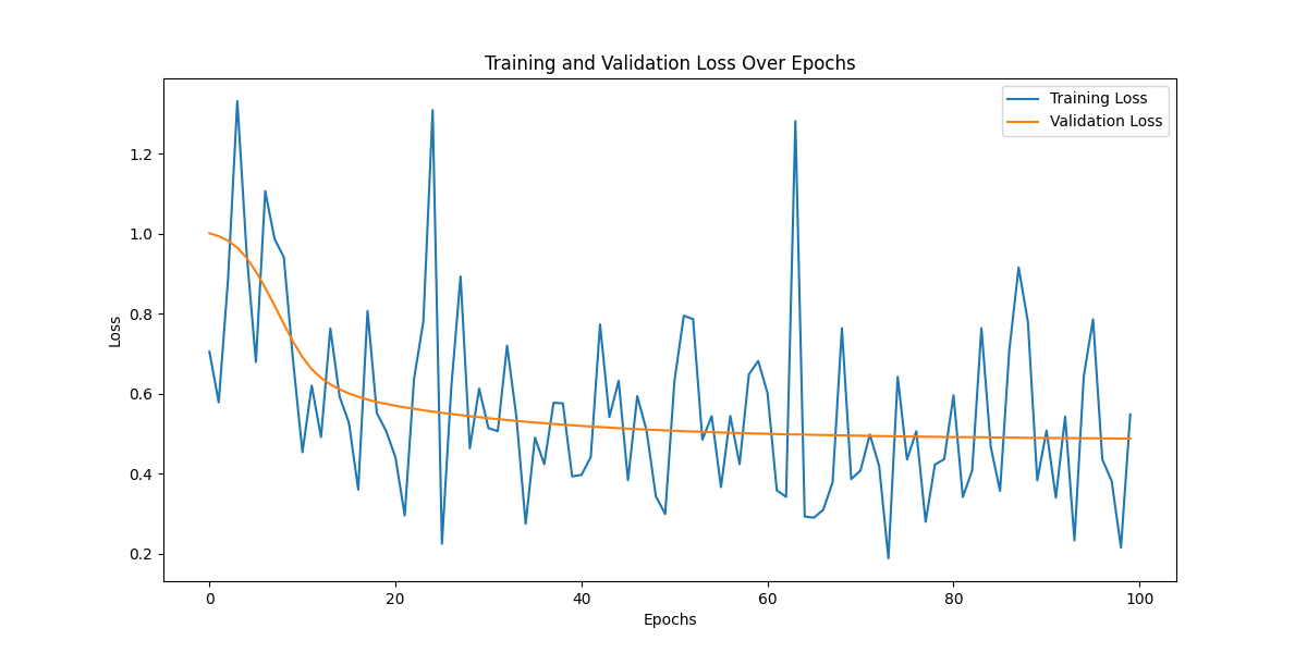
Liam leaned in to better look at the graph displayed on the screen. “So this is what you meant by visualizing the numbers, huh?”

Olivia nodded, pointing to the fluctuating blue line. “Exactly. See the blue line? That’s the Training Loss. As the model goes through the epochs, you can notice its peaks and troughs. It’s a bit erratic, but that’s not uncommon in training.”

Liam’s eyes followed the curve. “And the orange line?”

“That’s the Validation Loss,” Olivia explained. “Notice how it’s relatively smoother and trends downward over time? That suggests our model was converging, learning to generalize from the data rather than just memorizing it.”

Liam grinned, “Watching this unfold graphically is indeed more insightful. It’s like watching the model’s heartbeat, erratic at first, but finding its rhythm eventually.”

Olivia smiled in agreement, “Precisely! It’s always rewarding to see a model mature and stabilize over time.”

Forecasting the Grand Finale

With palpable excitement, Liam inquired, “Now that we’ve trained the model, can we use it to forecast the results for the upcoming Abu Dhabi Grand Prix 2023? I’m particularly keen on seeing how Sainz might fare.”

Olivia nodded, “Absolutely, but first, we must ensure that our prediction data is structured identically to our training data. Remember when we incorporated the starting position for training? We’d only know that after the qualifiers.”

Liam raised an eyebrow, “So what’s the workaround?”

Olivia explained, “We could make a hypothesis. Alternatively, we can simulate predictions for all potential starting positions for Sainz, from 1 to 20.”

She then shared the code:

def create_upcoming_race_data_for_positions(): 
    data = { 
        'start_position': list(range(1, 23)),  # Starting positions from 1 to 22 
        'year': [2023] * 22, 
        'month': [10] * 22, 
        'day': [8] * 22, 
        'circuit': ['Losail International Circuit'] * 22, 
        'name': ['Carlos Sainz'] * 22, 
        'constructor': ['Ferrari'] * 22 
    } 
 
    return pd.DataFrame(data) 
 
def predict_upcoming_races(predictor, upcoming_race_data, scalers, encoder): 
    # Step 1: Prepare and process upcoming race data 
    processed_upcoming_data = apply_one_hot_encoding(encoder, upcoming_race_data, 
                                                     ['circuit', 'name', 'constructor']) 
 
    for col in ['start_position', 'year', 'month', 'day']: 
        processed_upcoming_data[col] = scalers[col].transform(upcoming_race_data[col].values.reshape(-1, 1)) 
 
    processed_upcoming_data = processed_upcoming_data.astype({col: 'int' for col in processed_upcoming_data.select_dtypes(['bool']).columns}) 
 
    # Step 2: Convert to Tensor 
    upcoming_race_tensor = convert_to_tensor(processed_upcoming_data) 
 
    # Step 3: Create DataLoader 
    upcoming_race_loader = DataLoader(upcoming_race_tensor, batch_size=64, shuffle=False) 
 
    # Step 4: Run Inference 
    predictor.eval() 
    predictions = [] 
    with torch.no_grad(): 
        for batch in upcoming_race_loader: 
            outputs = predictor(batch) 
            predictions.extend(outputs) 
 
    # Step 5: Interpret Results 
    # Convert predictions to a format that can be understood, if necessary 
 
    return predictions

Liam absorbed the code and its implications. “Alright, let’s get this going. The anticipation is through the roof!”

Olivia activated the predictions, and a series of results populated the screen. She presented them to Liam, “Take a look.”

Liam’s eyes widened as he scanned through the output. “Wait, what? Even if Sainz is on pole position, he’s predicted to finish fifth?”

With a calming gesture, Olivia replied, “It’s essential to remember, Liam, these are just model predictions. There’s always a degree of uncertainty.”

Liam glanced at the screen, reading out:

Starting Position: 1, Predicted Finish: 5 
Starting Position: 2, Predicted Finish: 5 
Starting Position: 3, Predicted Finish: 5 
... 
Starting Position: 20, Predicted Finish: 12 
Starting Position: 21, Predicted Finish: 12 
Starting Position: 22, Predicted Finish: 12

Liam exhaled, “Well, I hope our model isn’t an oracle. We’ll see come race day!”

With a determined look, he asked, “Olivia, is there any way we can improve the accuracy of this model?”

Olivia leaned back, thinking for a moment. “Absolutely, Liam. Model improvement is an ongoing process. Here are a few strategies we can consider:

1. More Data: We can gather more historical race data, possibly extending our dataset to earlier seasons. A larger dataset can improve the generalization of our model.
2. Feature Engineering: We can introduce more relevant features. For example, understanding track-specific characteristics or weather conditions during races can be crucial.
3. Model Architecture: We could experiment with different architectures or try ensemble methods, combining the predictions from multiple models.
4. Hyperparameter Tuning: Adjusting learning rates, batch sizes, or other hyperparameters might improve performance.
5. Regularization Techniques: Implementing dropout or weight decay techniques can help reduce overfitting, making our model more robust.
6. Cross-Validation: Instead of a single train-test split, k-fold cross-validation can better understand how well our model might perform on unseen data.

Liam nodded, absorbing the information. “Alright, let’s get started then. We’ve got some work ahead of us!”

Olivia stretched her arms, yawning slightly. The weight of the day’s work began showing on her face.

“You know, Liam,” she began with a tired smile, “I think we’ve done enough for today. We’ve laid a solid foundation, and there will always be room for improvement. But sometimes, we must step back and see how things unfold.”

Liam nodded, appreciating her perspective. “You’re right. We’ve delved deep into the data and the model. It’s time to see how our predictions stack up against reality.”

She glanced at the clock, realizing the race was about to start. “Speaking of which, the Abu Dhabi Grand Prix is about to kick off. How about we grab snacks, put our feet up, and enjoy the race? We can always return to the drawing board later.”

Liam grinned, “Sounds like a plan. After all, amidst all these predictions and models, we shouldn’t forget the thrill of the race itself!”

The two left the room, excited chatter about the race filling the air, reminding themselves that sometimes, it’s all about the journey and not just the destination.

Conclusion

As the hours ticked away, anticipation for the Abu Dhabi Grand Prix peaked. Liam and Olivia, after their intense day of predictive modeling, eagerly turned their attention to the race, waiting to see how their predictions would fare against reality.

However, in a twist of fate, Carlos Sainz didn’t even make it to the starting grid. Due to unforeseen technical issues with his car, Sainz was ruled out of the race, shocking fans and analysts. The very premise of their predictions had been upended in an unexpected turn of events.

Olivia sighed, “It’s a stark reminder of the unpredictability of sports and life in general. No matter how advanced our models become, variables will always be outside our control.”

Liam nodded, “Indeed. Today, the real world gave us a lesson in humility.”

The two settled into their seats, focusing on the race that unfolded before them. Despite the hiccup in their predictive journey, the thrill of the sport remained undiminished. The roar of the engines, the strategies in play, and the sheer unpredictability of it all served as a fitting end to their day.

Olivia has made the source code available on GitHub for those interested in the intricacies of the model they developed. The “F1-predictor” repository provides a detailed walkthrough of their predictive journey.

GitHub - PatrickKalkman/F1-predictor: A repository that contains all the examples that go with a…

A repository that contains all the examples that go with a Medium article about creating a deep neural network using…

One thing was sure in the world of analytics and predictions: the authentic charm lies in the unexpected. The day may not have gone as planned, but it reinforced the idea that sometimes, the journey is more enlightening than the destination.

Join us on this journey: We invite readers to dive into the world of F1 predictive modeling. Explore the code, experiment with the models, and share your findings. Whether you’re a seasoned data scientist, an aspiring machine learning enthusiast, or just a fan of Formula 1, your contributions and insights are valuable.