AI Agent for Smart Home Climate Control: Harnessing Botanical Strategies for Energy Efficiency

Have you ever wondered how greenhouses achieve such remarkable energy efficiency? The secret lies in using strategies like daily temperature integration, which ensures ideal plant growth conditions and optimal energy use.

For instance, consider cucumbers: they grow best at an average temperature of around 22 °C. Daily temperature integration allows for temperature variations during the day as long as the average temperature remains around 22 °C.

This method not only promotes healthy growth but also optimizes energy consumption. Integrating this knowledge with energy prices and weather forecasts can significantly reduce energy usage, costs, and environmental impact.

This integration is precisely what modern climate control systems aim to achieve. Many systems include features such as ‘Temperature Optimization,’ which apply these principles to enhance efficiency.

In this article, we’ll explore how to implement an AI agent using LangGraph that leverages temperature integration principles similar to those used in greenhouses to manage energy efficiently in our homes.

This AI-driven climate control system can automatically adjust temperatures, optimizing energy use while keeping our living spaces comfortable.

The complete source code of the AI Agent is available on GitHub, including a demo mode that uses cached data.

Table of Contents

· The Core Components of Our AI Agent
∘ Energy Price Retriever
∘ Weather Forecast Retriever
∘ Current Temperature Retriever
∘ Optimal Temperature Calculator
∘ Decision Insight
∘ Temperature Setpoint Realizer
· Selecting our AI Agent framework
· LangGraph nodes and shared state
· 1. Energy prices node
· 2. Weather forecast node
· 3. Sensor Data Node
· 4. Optimal temperature calculator node
· 5. Decision insight node
· Temperature setpoint realizer node
· Putting it al together
· Running the Agent
∘ Installing dependencies
∘ Starting the agent
· What’s next?

The Core Components of Our AI Agent

Before diving into the code, let’s zoom out and look at the different modules that make up our AI Agent. We will describe each module from left to right.

Energy Price Retriever

This module is responsible for retrieving the current electricity prices, which are crucial for our AI Agent's operational strategy. The system can make informed decisions about adjusting indoor temperatures by accessing today’s hourly electricity prices via an API from enever.nl.

This functionality enables our system to increase the temperature when energy is cheaper and decrease it when it’s more costly.

Weather Forecast Retriever

This module retrieves the weather forecast, focusing specifically on expected hourly temperatures essential for effective climate control. By utilizing an API from WeatherAPI.com, our system gains access to accurate and up-to-date weather data.

This information is important as it helps the system predict and adapt to changing environmental conditions, ensuring optimal indoor temperature settings.

The hourly temperature data directly informs our Optimal Temperature Calculator, enabling it to adjust real-time settings for enhanced energy efficiency and occupant comfort.

Current Temperature Retriever

This module acquires the current room temperature, which is also critical for our climate control strategy. It interacts with a Google Nest thermostat through the Google Device Console API, ensuring our system has real-time temperature data.

This allows the AI Agent to make immediate adjustments based on indoor conditions, aligning these with pre-determined setpoints from the Optimal Temperature Calculator.

The continuous update of room temperature ensures that our system can maintain optimal comfort levels efficiently, adapting dynamically to both programmed settings and unexpected temperature variations.

Optimal Temperature Calculator

This module contains the algorithm for calculating the optimal temperature for each hour, utilizing daily temperature integration and the data from the preceding modules. The algorithm operates through a series of steps:

1. Assess Current Situation

• Evaluate the difference between the current indoor temperature and the desired average temperature to establish the baseline for adjustments.
• Gather and process data on hourly electricity prices, weather forecasts, sensor readings, and other relevant parameters.

2. Predict Temperature Shifts

• Forecast how the indoor temperature would naturally evolve without intervention, considering the differential between indoor and outdoor temperatures.
• Adjust for factors such as insulation and ambient temperature to refine predictions.

3. Calculate Adjustments

• Determine necessary heating or cooling adjustments to maintain the indoor temperature within a targeted range around the desired average temperature.
• Use dynamic bandwidth, adjusted for electricity price volatility, to calculate minimum and maximum setpoints for each hour.

4. Compute Costs and Optimize

• Normalize electricity prices and calculate initial setpoints based on various factors, including price fluctuations and weather forecasts.
• Compute the costs associated with each potential adjustment, factoring in fluctuating hourly energy prices.
• Evaluate various adjustment strategies and their timings to identify the most cost-effective approach that maintains the desired temperature.

5. Minimize Total Costs

• Adjust setpoints to ensure they remain within the acceptable comfort range while aligning with the desired average temperature.
• Select the strategy that minimizes total energy costs throughout the day, ensuring optimal temperature management and energy efficiency.

The module produces setpoints with corresponding times, baseline and optimized costs, and potential savings, facilitating efficient and comfortable indoor climate control.

Decision Insight

This module enhances the transparency and understandability of our AI Agent by articulating the reasoning behind each hourly temperature setpoint. It is critical to increase user trust by providing clear, understandable explanations of the system’s decisions.

Example Explanation: Consider a scenario where the optimal indoor temperature is set higher than the previous hour:

• Context: At 3 PM, the outdoor temperature is forecasted to drop sharply. Without intervention, the indoor temperature would decrease to an uncomfortable 18°C, below the comfortable minimum of 20°C set for today.
• Decision Rationale: To maintain comfort and minimize heating costs during this peak price hour, the system preemptively increases the indoor temperature by one °C earlier than usual. This proactive adjustment helps avoid more significant, costly heating later, thus aligning with our strategy to balance comfort with efficiency.
• Cost Implications: Although this adjustment occurs during a higher energy price window, it prevents more significant temperature corrections when energy prices peak, resulting in overall cost savings throughout the day.

We will use an LLM to explain the decisions made by the Optimal Temperature Calculator. It summarizes the hourly temperature setpoints and the rationale behind each setpoint.

Temperature Setpoint Realizer

This module is the final step in our climate control process. It implements the temperature strategies calculated by the Optimal Temperature Calculator.

It communicates directly with the thermostat to set the optimal hourly temperature based on the most energy-efficient and cost-effective calculations previously determined. The Temperature Setpoint Realizer uses the interface with the Google Nest thermostat via the Google Device Console API.

Selecting our AI Agent framework

For the development of this AI Agent, I chose to continue using LangGraph, a robust Agent framework provided by LangChain. My previous experiences with LangGraph were highly positive, mainly due to its versatile architecture, which lets you integrate normal Python functions.

LangGraph is designed to separate the system into multiple nodes, each sharing and interacting through a common state object. This architecture allows for efficient information exchange where each node can read from and contribute to the shared state.

This feature mainly benefits our project as it supports seamless integration and synchronization between different modules.

Given our system’s structure, where each module performs distinct yet interconnected functions, LangGraph’s node-based approach aligns perfectly. Our previously designed modules can be easily adapted into LangGraph nodes, facilitating a modular and scalable system architecture.

This not only simplifies development but also enhances the overall robustness and maintainability of our climate control AI Agent.

LangGraph nodes and shared state

Each previously described module in our system is converted into a LangGraph node, facilitating better integration and data sharing.

A ‘Shared State’ is a central repository for each node to access and update. This shared state is pivotal to the system’s efficiency as it consolidates critical data, including:

• Energy Prices Per Hour: Updated once daily, these prices allow the system to make cost-effective adjustments.
• Expected Temperature Per Hour: Forecasted temperatures inform our predictive adjustments.
• Current Temperature: Real-time temperature data ensures our responses are timely and appropriate.
• Optimal Temperature Setpoint Per Hour: The culmination of input from the other nodes, these setpoints are calculated to ensure optimal comfort and energy efficiency.

We are now ready to start implementing our AI agent. We will describe each node in a separate section.

1. Energy prices node

This node is responsible for retrieving hourly energy prices, specifically electricity prices. For this purpose, we utilize Enever.nl, a website that provides hourly energy prices for several Dutch energy providers, including my provider, Eneco.

It’s important to note that Enever specifies that its data cannot be used for commercial purposes and enforces a strict request limit of 250 API calls per month. To stay within these constraints, our system retrieves the data once per day and caches it using files.

To access their API, you need to obtain a token from their website, which our Agent reads from an environment variable.

Here is the function that constitutes the energy prices node. It uses the get_energy_prices function to fetch data from Enever.nl. The argument electricity_price_today specifies the type of energy prices we want:

def energy_prices_node(state): 
    prices = get_energy_prices('electricity_price_today') 
    if prices is None: 
        return {"error": "Data not available"} 
    energy_prices_per_hour = transform_data(prices) 
    return {"energy_prices_per_hour": energy_prices_per_hour}

The data retrieved looks like this (sample for two hours; the actual response contains 24 hours):

[ 
    { 
        "datum": "2024-05-13 00:00:00", 
        "prijs": "0.027120", 
        "prijsAA": "0.185665", 
        "prijsAIP": "0.194715", 
        "prijsANWB": "0.212865", 
        "prijsBE": "0.185455", 
        "prijsEE": "0.191315", 
        "prijsEN": "0.185055" 
     }, 
     { 
        "datum": "2024-05-13 01:00:00", 
        "prijs": "0.026080", 
        "prijsAA": "0.184407", 
        "prijsAIP": "0.193457", 
        "prijsANWB": "0.211607", 
        "prijsBE": "0.184197", 
        "prijsEE": "0.190057", 
        "prijsEN": "0.183797" 
      } 
]

The transform_data function extracts the relevant electricity price for Eneco (prijsEN) and the corresponding date-time, resulting in a structure like this:

[{'date': '2024-05-13T00:00:00', 'price': '0.185055'},  
 {'date': '2024-05-13T01:00:00', 'price': '0.183797'}, 
 {'date': '2024-05-13T02:00:00', 'price': '0.183506'}]

The get_energy_prices function implements caching to reduce API calls. It first checks for a cached file; if found, it loads the data from the file. Otherwise, it uses the Python requests library to fetch the JSON from Enever:

def get_energy_prices(data_type): 
    if data_type == "electricity_price_tomorrow" and datetime.datetime.now().hour < 16: 
        logger.info(f"Data for {data_type} not yet available. Skipping.") 
        return None 
 
    ensure_directory_exists(ENERGY_CACHE_DIR) 
    cache_file_path = get_cache_file_path(data_type) 
    cached_data = load_data_from_cache(cache_file_path) 
 
    if cached_data: 
        logger.info(f"Using cached data for {data_type}.") 
        return cached_data 
 
    url = get_api_url(data_type) 
    try: 
        prices = fetch_data_from_api(url) 
        save_data_to_cache(cache_file_path, prices) 
        return prices 
    except Exception as e: 
        logger.error(f"An error occurred while getting energy prices for {data_type}: {e}") 
        return None

Check GitHub for the source of the complete node.

2. Weather forecast node

The weather forecast node is designed to pull hourly temperature data for a specific location, which is crucial for our AI Agent’s temperature management strategy.

This node utilizes WeatherAPI, which requires an API key to access forecast data. After obtaining and securely storing the API key in our environment settings, we can make requests to WeatherAPI’s endpoint.

An API call to https://api.weatherapi.com/v1/forecast.json retrieves a comprehensive set of weather-related data. Our system extracts only the hourly temperature forecasts needed for our operations from this dataset.

The code snippet below outlines the weather_forecast_node's process of fetching and transforming the weather data into a usable format for the current day:

def weather_forecast_node(state): 
    url = get_api_url() 
    forecast = fetch_data_from_api(url) 
    if forecast is None: 
        return {"error": "Data not available"} 
    transformed_forecast = transform_forecast_data(forecast) 
    return {"weather_forecast": transformed_forecast} 
 
 
def fetch_data_from_api(url): 
    try: 
        response = requests.get(url) 
        response.raise_for_status() 
        data = response.json() 
        return data['forecast']['forecastday'][0]['hour'] 
    except requests.HTTPError as e: 
        logger.error(f"HTTP error occurred: {e}") 
        return None 
    except requests.RequestException as e: 
        logger.error(f"Request exception occurred: {e}") 
        return None 
 
 
def transform_forecast_data(forecast): 
    transformed_data = [] 
    for entry in forecast: 
        date_iso = datetime.datetime.strptime(entry["time"], "%Y-%m-%d %H:%M").isoformat() 
        transformed_data.append({ 
            "date": date_iso, 
            "temperature": entry["temp_c"] 
        }) 
    return transformed_data 
 
 
def get_api_url(): 
    api_key = os.getenv("WEATHER_API_KEY") 
    location = os.getenv("LOCATION") 
    current_date = datetime.date.today() + datetime.timedelta(days=1) 
    formatted_date = current_date.strftime('%Y-%m-%d') 
    return f"{API_BASE_URL}?q={location}&days=1&dt={formatted_date}&key={api_key}"

Transforming the data involves processing the JSON response from WeatherAPI to extract only the essential information needed for our AI Agent. This step focuses on two key aspects:

1. Date and Time Conversion: The datetime information from the JSON is converted into a standard datetime format. This ensures that the timing of the weather data aligns precisely with our system’s scheduling needs.
2. Temperature Data Extraction: We retain the temperature data for each hour. This selective extraction simplifies the JSON structure, making the data easier to manage and integrate into our system.

def fetch_data_from_api(url): 
    try: 
        response = requests.get(url) 
        response.raise_for_status() 
        data = response.json() 
        return data['forecast']['forecastday'][0]['hour'] 
    except requests.HTTPError as e: 
        logger.error(f"HTTP error occurred: {e}") 
        return None 
    except requests.RequestException as e: 
        logger.error(f"Request exception occurred: {e}") 
        return None 
 
 
def transform_forecast_data(forecast): 
    transformed_data = [] 
    for entry in forecast: 
        date_iso = datetime.datetime.strptime(entry["time"], "%Y-%m-%d %H:%M").isoformat() 
        transformed_data.append({ 
            "date": date_iso, 
            "temperature": entry["temp_c"] 
        }) 
    return transformed_data

Finally, the node packages this streamlined weather data into a weather_forecast field. This field contains the forecasted temperatures for each hour, formatted as follows:

[ 
  {'date': '2024-05-16T00:00:00', 'temperature': 13.6},  
  {'date': '2024-05-16T01:00:00', 'temperature': 13.3},  
  {'date': '2024-05-16T02:00:00', 'temperature': 12.9},  
  {'date': '2024-05-16T03:00:00', 'temperature': 12.6},  
  {'date': '2024-05-16T04:00:00', 'temperature': 12.9}, 
  .... 
]

Here on GitHub, you can find the source code of the complete node.

3. Sensor Data Node

To retrieve data from your Google Nest thermostat, you must set up accounts and create a project within Google’s Device Access Console to access their API. You’ll need the following information:

• Access Token and Refresh Token: Authorize your software to access thermostat data.

• Client ID and Client Secret: Identify your application to Google.

• Project ID and Device Name: Identify the specific project and device you want to access.

With this information, the sensor_data_node can connect to the Google Nest API. While our primary interest is temperature, we also fetch additional data points such as humidity and current thermostat settings.

Since the access token is only valid for one hour, a mechanism stores the access token and its expiration time. When the token expires, the system automatically requests a new one using the refresh token.

def sensor_data_node(state): 
    device_info = get_device_info() 
    if device_info: 
        extracted_traits = extract_device_traits(device_info) 
        return {'sensor_data': extracted_traits} 
    return {'error': 'Data not available'} 
 
 
def get_device_info(): 
    try: 
        access_token = get_access_token() 
    except Exception as e: 
        logger.error(f'Failed to get access token: {e}') 
        return None 
 
    device_name = os.getenv('DEVICE_NAME') 
    url = f'https://smartdevicemanagement.googleapis.com/v1/{device_name}' 
    headers = {'Authorization': f'Bearer {access_token}'} 
    response = requests.get(url, headers=headers) 
    if response.status_code == 401: 
        logger.error('Authentication required. Please re-authenticate.') 
        return None 
 
    if response.status_code != 200: 
        logger.error(f'Failed to get device info. Status code: {response.status_code}') 
        return None 
 
    return response.json() 
 
 
def extract_device_traits(device_info): 
    traits = device_info.get("traits", {}) 
    heat_celsius = traits.get("sdm.devices.traits.ThermostatEco", {}).get("heatCelsius") 
    status = traits.get("sdm.devices.traits.ThermostatHvac", {}).get("status") 
    ambient_temperature_celsius = traits.get("sdm.devices.traits.Temperature", {}).get("ambientTemperatureCelsius") 
    thermostat_mode = traits.get("sdm.devices.traits.ThermostatMode", {}).get("mode") 
    connectivity_status = traits.get("sdm.devices.traits.Connectivity", {}).get("status") 
    humidity = traits.get("sdm.devices.traits.Humidity", {}).get("ambientHumidityPercent") 
 
    return { 
        "heat_celsius": heat_celsius, 
        "humidity": humidity, 
        "ambient_temperature_celsius": ambient_temperature_celsius, 
        "thermostat_mode": thermostat_mode, 
        "status": status, 
        "connectivity_status": connectivity_status 
    }

Here you can find the source code of the Sensor Data Node.

4. Optimal temperature calculator node

The Optimal Temperature Calculator Node calculates the optimal temperature setpoints for each hour of the day, ensuring that the average indoor temperature stays within a predefined bandwidth and averages to the desired set temperature over 24 hours.

The node performs its calculations using the following data from the state:

• Hourly Energy Prices
• Weather Forecast
• Sensor Data
• Bandwidth
• Temperature Setpoint
• Insulation Factor

The node calculates the hourly setpoints and the savings compared to baseline costs. We use Numpy arrays to make the calculations more efficient.

def optimal_temperature_calculator_node(state): 
    electricity_prices_data = state['energy_prices_per_hour'] 
    weather_forecast_data = state['weather_forecast'] 
    sensor_data = state['sensor_data'] 
    bandwidth = state['bandwidth'] 
    temperature_setpoint = state['temperature_setpoint'] 
    insulation_factor = state['insulation_factor'] 
 
    electricity_prices = np.array([float(item['price']) for item in electricity_prices_data]) 
    weather_forecast = np.array([item['temperature'] for item in weather_forecast_data]) 
    current_temperature = sensor_data.get('ambient_temperature_celsius') 
 
    setpoints = calculate_setpoints(electricity_prices, weather_forecast, temperature_setpoint, 
                                    bandwidth, current_temperature, insulation_factor) 
    setpoints_with_time = add_datetime_to_setpoints_and_round_setpoints(setpoints) 
    baseline_cost, optimized_cost, savings = calculate_costs(setpoints, electricity_prices, 
                                                             weather_forecast, temperature_setpoint) 
 
    return { 
        "setpoints": setpoints_with_time, 
        "baseline_cost": baseline_cost, 
        "optimized_cost": optimized_cost, 
        "savings": savings 
    }

calculate_setpoints

The calculate_setpoints function determines the optimal setpoints. It adjusts the bandwidth dynamically based on the volatility of electricity prices and normalizes these prices for further calculations.

def calculate_setpoints(electricity_prices, weather_forecast, temperature_setpoint, 
                        bandwidth, current_temperature, insulation_factor): 
 
    volatility = np.std(electricity_prices) / np.mean(electricity_prices) 
    dynamic_bandwidth = bandwidth * (1 + volatility) 
 
    min_setpoint = temperature_setpoint - dynamic_bandwidth / 2 
    max_setpoint = temperature_setpoint + dynamic_bandwidth / 2 
 
    normalized_prices = normalize_prices(electricity_prices) 
 
    setpoints = np.array([ 
        calculate_initial_setpoint(temperature_setpoint, min_setpoint, max_setpoint, 
                                   normalized_prices[hour], weather_forecast[hour], 
                                   current_temperature, insulation_factor) 
        for hour in range(24) 
    ]) 
 
    setpoints = adjust_setpoints(setpoints, temperature_setpoint, min_setpoint, max_setpoint) 
 
    final_average = round(np.mean(setpoints), 2) 
    if abs(final_average - temperature_setpoint) > 0.5: 
        logger.info(f"Adjusted setpoints outside ±0.5°C range. {final_average} != {temperature_setpoint}") 
 
    return setpoints

Supporting Functions

1. normalize_prices: Normalizes electricity prices to a 0-1 scale to standardize the impact of price fluctuations.

def normalize_prices(electricity_prices): 
    min_price = np.min(electricity_prices) 
    max_price = np.max(electricity_prices) 
    return (electricity_prices - min_price) / (max_price - min_price)

2. calculate_initial_setpoint: Calculates the initial setpoint for each hour by adjusting for electricity prices, weather, and insulation.

def calculate_initial_setpoint(average_setpoint, min_setpoint, max_setpoint, price_factor, 
                               outside_temp, current_temperature, insulation_factor): 
    ideal_setpoint = average_setpoint + (max_setpoint - min_setpoint) * (0.75 - price_factor) * 2 
 
    temp_adjustment = insulation_factor * (0.1 * (average_setpoint - outside_temp) if outside_temp < average_setpoint else -0.1 * (outside_temp - average_setpoint)) 
    ambient_adjustment = 0.05 * (average_setpoint - current_temperature) if current_temperature < average_setpoint else -0.05 * (current_temperature - average_setpoint) 
 
    ideal_setpoint += temp_adjustment + ambient_adjustment 
    return np.clip(ideal_setpoint, min_setpoint, max_setpoint)

3. adjust_setpoints: Ensures the setpoints average out to the desired temperature.

def adjust_setpoints(setpoints, average_setpoint, min_setpoint, max_setpoint): 
    current_average = np.mean(setpoints) 
    adjustment_needed = average_setpoint - current_average 
 
    adjusted_setpoints = setpoints + adjustment_needed 
    return np.clip(adjusted_setpoints, min_setpoint, max_setpoint)

Result

When we combine all the data and the calculated setpoint and plot this in a graph, we see the following:

The graph illustrates the temperature setpoints, weather forecast, and scaled electricity prices over 24 hours. The function that generates this graph can be found here on GitHub.

This visualization highlights how the algorithm adjusts the indoor temperature setpoints in response to changing electricity prices and outdoor temperatures.

When energy prices are lower, the setpoints are adjusted to higher temperatures to take advantage of the lower costs. Conversely, when energy prices rise, the setpoints are lowered to save on heating costs.

This adjustment ensures the indoor temperature remains comfortable while optimizing for cost savings.

By implementing this approach, significant savings can be achieved without compromising on comfort. The calculated setpoints help minimize energy usage during peak price periods and make the most of off-peak hours.

5. Decision insight node

The Decision insight node explains the reasoning behind each hourly temperature setpoint. Understanding the logic behind automated decisions is increasingly important as systems become more complex.

This is particularly true for complex systems such as climate control systems, which have significant room for improvement in transparency and user understanding.

Our AI Agent addresses this by leveraging a Large Language Model (LLM) to explain the reasoning based on the input and calculated data. This functionality adds a layer of interpretability to the system, allowing users to understand why certain temperature setpoints were chosen at specific times.

I chose Groq for this task, a company specializing in generative AI solutions and the creator of the LPU™ Inference Engine. Groq’s custom hardware enables fast inference, making it ideal for real-time applications like ours.

After experimenting with various models, I found that the Llama 3 70B with an 8K Context Length provided the best results.

Below, you’ll find the implementation of the decision_insight_node. This node utilizes the langchain groq PyPI package to interact with the Groq API.

It extracts all necessary data from the state and constructs a prompt for the LLM. The LangChain Expression Language (LCEL) is used to build the generator, facilitating the interaction between the prompt and the LLM.

def decision_insight_node(state): 
    if state.get('mode') == 'demo': 
        return {"explanation": ("The temperature at 10:00:00 is set to 22.28 degrees because the electricity prices are" 
                                "relatively low at this time, and the weather is warm with a forecasted temperature" 
                                " of 18.8°C. Additionally, the average temperature over the 24-hour period should be" 
                                " within the bandwidth range of 6.0°C, which allows for some flexibility in " 
                                "temperature adjustments to optimize energy costs. By setting the temperature to " 
                                "22.28°C, the system is taking advantage of the low energy prices while maintaining " 
                                "a comfortable temperature and staying within the desired bandwidth.")} 
 
    GROQ_LLM = ChatGroq(model=MODEL_NAME) 
 
    explain_calculated_setpoints_prompt = PromptTemplate( 
        template="""\ 
        system 
        You are an expert in energy management and explaining the calculated temperature setpoints. 
 
        user 
        Given the following data: 
        - Energy prices per hour: {energy_prices} 
        - Weather forecast: {weather_forecast} 
        - Sensor data: {sensor_data} 
        - Calculated setpoints: {setpoints} 
        - Bandwidth: {bandwidth} 
        - Temperature setpoint: {temperature_setpoint} 
        - Insulation factor: {insulation_factor} 
 
        Explain why the temperature at {hour}:00 is set to {setpoint} degrees. Give a brief explanation. 
        For example, 'The temperature is set the lower limit of {setpoint} degrees celcius because the electricity 
        prices are high and the weather is cold.' Or 
        'The temperature is set to the higher limit of {setpoint} degrees celcius because the electricity prices are 
        low and the weather is warm.' 
        Also consider that the average temperature should be within the bandwidth range over 24 hours. 
 
        assistant""", 
        input_variables=["energy_prices", "weather_forecast", "sensor_data", 
                         "setpoints", "bandwidth", "temperature_setpoint", 
                         "insulation_factor", "hour", "setpoint"], 
    ) 
 
    explanation_generator = explain_calculated_setpoints_prompt | GROQ_LLM | StrOutputParser() 
    hour = round(time() / 3600) % 24 
    setpoint = state["setpoints"][hour] 
    explanation = explanation_generator.invoke({ 
        "energy_prices": state["energy_prices_per_hour"], 
        "weather_forecast": state["weather_forecast"], 
        "sensor_data": state["sensor_data"], 
        "setpoints": state["setpoints"], 
        "bandwidth": state["bandwidth"], 
        "temperature_setpoint": state["temperature_setpoint"], 
        "insulation_factor": state["insulation_factor"], 
        "hour": hour, 
        "setpoint": setpoint["setpoint"], 
    }) 
 
    logger.info(f"Explanation for {hour}:00: {explanation}") 
 
    return {"explanation": explanation}

The decision_insight_node initializes the Groq LLM model and constructs a prompt template with placeholders for all relevant data.

It then generates an explanation for the current hourly by invoking the LLM with the prepared data and logging the generated explanations.

The final output is a generated explanation stored in the state.

Below, you see an example of a generated explanation.

The temperature at 10:00:00 is set to 22.28 degrees because the electricity prices are relatively low at this time, and the weather is warm, with a forecasted temperature of 18.8°C.

Additionally, the average temperature over the 24-hour period should be within the bandwidth range of 6.0°C, which allows for some flexibility in temperature adjustments to optimize energy costs.

By setting the temperature to 22.28°C, the system takes advantage of the low energy prices while maintaining a comfortable temperature and staying within the desired bandwidth.

I believe there’s still room for improvement in the prompt, but it’s effective for now.

Temperature setpoint realizer node

The final node in our AI Agent is the Temperature setpoint realizer node, which applies the calculated setpoints to our thermostat — in this case, a Google Nest.

This node retrieves the current hour’s setpoint from the state and sends a POST request to the thermostat to adjust the temperature accordingly.

As with retrieving sensor data from the Google Nest, you need an access token to authenticate your request. This token ensures that only authorized users can adjust the thermostat settings.

Below is a snippet of the Python code for the temperature_setpoint_realizer_node, focusing on the part where it retrieves the current hour’s setpoint and sends the POST request.

def temperature_setpoint_realizer_node(state): 
    current_hour = round(time() / 3600) % 24 
    setpoints = state['setpoints'] 
    temperature_setpoint = setpoints[current_hour]['setpoint'] 
    set_calculated_temperature(temperature_setpoint) 
 
 
def set_calculated_temperature(temperature_setpoint): 
    try: 
        access_token = get_access_token() 
    except Exception as e: 
        logger.error(f'Failed to get access token: {e}') 
        return None 
 
    device_name = os.getenv('DEVICE_NAME') 
    url = f'https://smartdevicemanagement.googleapis.com/v1/{device_name}:executeCommand' 
    headers = { 
        'Authorization': f'Bearer {access_token}', 
        'Content-Type': 'application/json' 
    } 
 
    data = { 
        "command": "sdm.devices.commands.ThermostatTemperatureSetpoint.SetHeat", 
        "params": { 
            "heatCelsius": temperature_setpoint 
        } 
    } 
 
    logger.info(f'Setting temperature to {temperature_setpoint} degrees') 
 
    response = requests.post(url, headers=headers, json=data) 
 
    if response.status_code == 401: 
        logger.error('Authentication required. Please re-authenticate.') 
        return None 
 
    if response.status_code != 200: 
        logger.error(f'Failed to set temperature. Status code: {response.status_code} reason: {response.json()}') 
        return None 
 
    return response.json()

The complete source code of the temperature_setpoint_realizer_node is available on GitHub.

Putting it together

Now that we have implemented all the nodes, we can use LangGraph to create the workflow in main.py.

First, we create a StateGraph instance and pass in our state,AgentState. Then, we add each node to the graph.

The add_node function expects two parameters:

• Key: A unique string representing the name of the node.
• Action: The action to be executed when this node is called. This can be a function or a runnable.

Next, we connect the nodes using edges. We set the entry point of the graph to the configuration_node and connect each subsequent node, ending with the temperature_setpoint_realizer_node connected to the END node, signaling the completion of the graph.

workflow = StateGraph(AgentState) 
workflow.add_node("configuration_node", configuration_node) 
workflow.add_node("energy_prices_node", energy_prices_node) 
workflow.add_node("weather_forecast_node", weather_forecast_node) 
workflow.add_node("sensor_data_node", sensor_data_node) 
workflow.add_node("optimal_temperature_calculator_node", optimal_temperature_calculator_node) 
workflow.add_node("decision_insight_node", decision_insight_node) 
workflow.add_node("temperature_setpoint_realizer_node", temperature_setpoint_realizer_node) 
 
workflow.set_entry_point("configuration_node") 
workflow.add_edge("configuration_node", "energy_prices_node") 
workflow.add_edge("energy_prices_node", "weather_forecast_node") 
workflow.add_edge("weather_forecast_node", "sensor_data_node") 
workflow.add_edge("sensor_data_node", "optimal_temperature_calculator_node") 
workflow.add_edge("optimal_temperature_calculator_node", "decision_insight_node") 
workflow.add_edge("decision_insight_node", "temperature_setpoint_realizer_node") 
workflow.add_edge("temperature_setpoint_realizer_node", END) 
app = workflow.compile() 
 
for s in app.stream({}): 
    result = list(s.values())[0] 
    logger.info(result)

After creating the graph, we compile it using the compile method. During this process, LangGraph validates the graph. If you forget to connect a node or properly terminate the graph, LangGraph will notify you during compilation.

Finally, we start the graph using the stream method, passing it an empty input. I use the stream method instead of invoke because it allows us to log the values returned from each node, which is helpful for tracing.

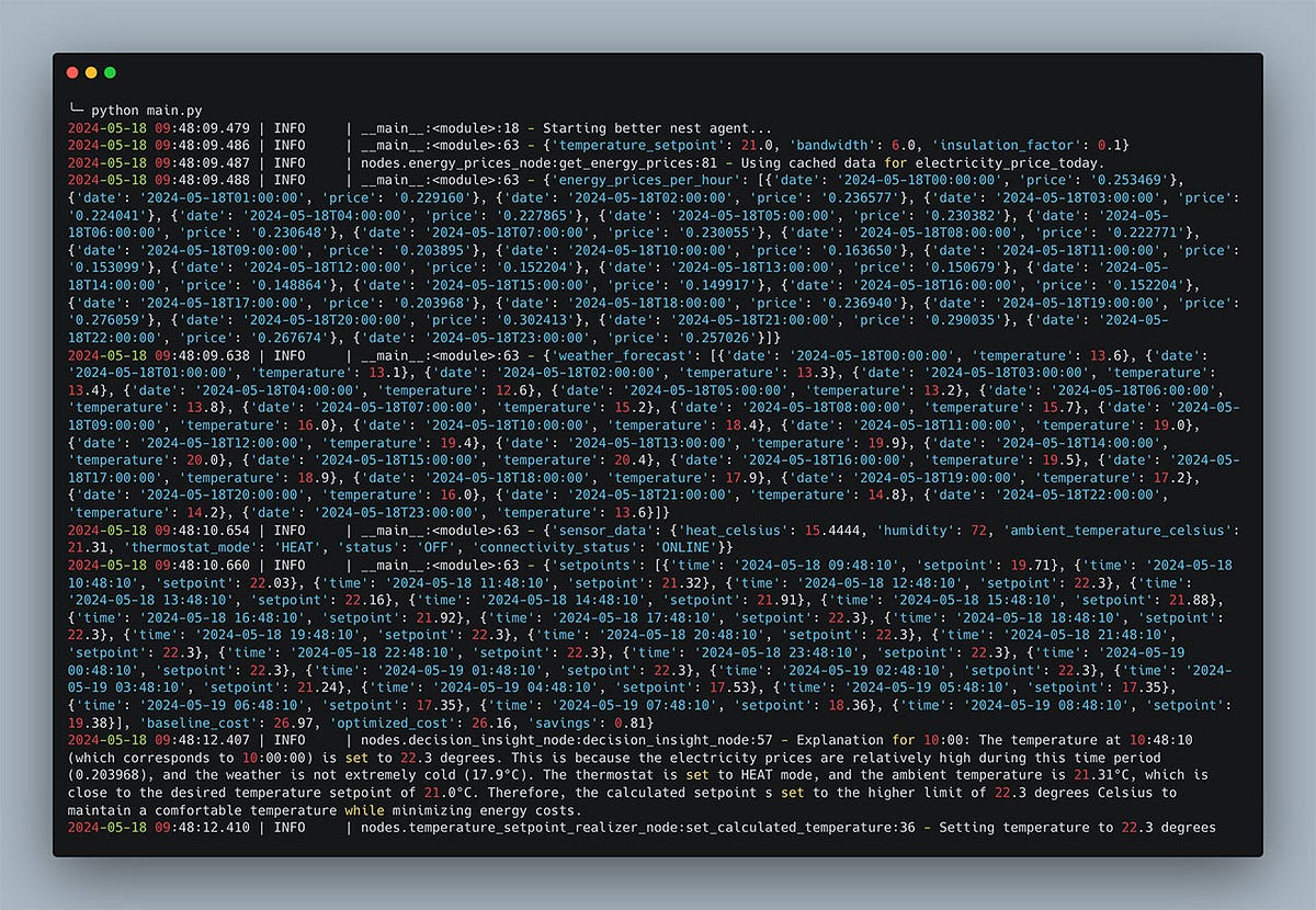
I use the loguru logging package to add logging for traceability, as shown in the screenshot below.

Running the Agent

The complete source code for the AI agent is available on GitHub. Below, you’ll find step-by-step instructions for configuring and running the agent on your local machine.

While running the program might require specific environment settings, some of which involve creating accounts to access necessary APIs, I’ve added a demo mode that allows you to run the agent using cached data.

By default, this demo mode is enabled. You can change it via the configuration_node, as shown below:

def configuration_node(state): 
    return { 
        "temperature_setpoint": 21.0, 
        "bandwidth": 6.0, 
        "insulation_factor": 0.1, 
        "mode": "demo" 
    }

To use live data instead of the demo mode, change the mode key to something other than "demo." Remember to set all the required environment variables as specified in the .env.example file.

Installing dependencies

The program uses various PyPi packages. Depending on your preference, you can install these dependencies via pip or conda.

Run one of the following command in your terminal to set up your environment:

pip install -r requirements.txt

conda env create -f environment.yml

Starting the agent

Once you’ve configured your environment and installed all dependencies, you can run the agent by executing the main script:

python main.py

What’s next?

What’s next for our AI agent? How can we push the boundaries further and enhance its capabilities? This was my second AI agent using LangGraph, and I find it increasingly versatile and powerful.

The Decision Insight module of this AI agent shows AI’s unique capabilities, particularly in explaining the rationale behind system actions. This transparency is invaluable for users seeking to understand and trust automated decisions.

Throughout the development of this AI agent, several ideas for enhancements emerged:

Energy Prices

• Incorporate Gas Prices: Integrate gas prices and calculate the energy required (gas or electricity) to increase the temperature by one degree Celsius. This would provide a more comprehensive view of energy costs and help optimize heating strategies.

Weather Forecast

• Radiation Prediction: Include expected solar radiation in the predictions. Solar radiation significantly impacts indoor temperatures, primarily through windows. Accounting for this can improve the accuracy of the temperature setpoints.

Optimal Temperature Calculator Improvements

• Advanced Scenarios: Enhance the calculation engine to simulate more realistic scenarios, allowing for more robust decision-making.
• Frequent Recalculations: Recalculate setpoints multiple times throughout the day to adapt to changing weather conditions and solar radiation levels.

Decision Insight

• Voice Integration: Enable the Decision Insight Module to provide explanations via voice, making the system more interactive and user-friendly.
• Real-Time Queries: Allow users to ask questions in real time rather than relying on pre-calculated responses. Maybe use an even more advanced model like GPT-4 from OpenAI.
• Prompt Optimization: Continuously refine the prompt and experiment with different models to enhance the quality of the insights provided.

But as always, my approach is First make it work, then make it right, and finally, optimize it.

Happy learning and coding!

This story is published on Generative AI. Connect with us on LinkedIn and follow Zeniteq to stay in the loop with the latest AI stories.

Subscribe to our newsletter to stay updated with the latest news and updates on generative AI. Let’s shape the future of AI together!